2D Cross Correlation

Dear ncl community,

I generate 2D spatial cross correlation at zero time lag between two near surface temperature fields obtained from two model runs using:

    ccr = esccr(ts1,ts2,mxlag)

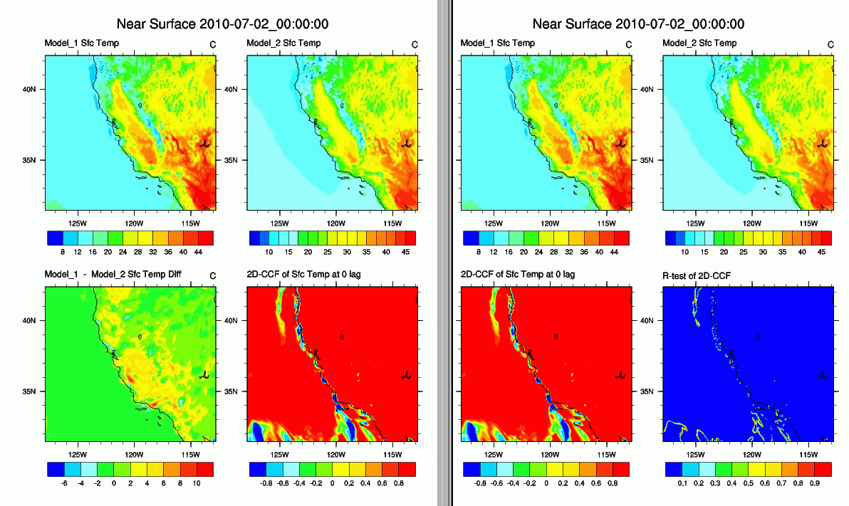
and trying to understand what it really shows. I attached a composite picture obtained from the screen dump of two .ps images, so both pictures can be examined simultaneously to evaluate my questions.

I extracted near surface temperature from two model runs and plotted on the top of a 4-panel plot next to each other. I also plotted the difference between these two fields and 2D spatial cross correlation of the two fields at zero lag time at the bottom portion of the 4 panel plot. In the second 4-panel plot within the same picture, I repeated the process but this time replaced the difference plot with the R-test plot to get another evaluation tool. The whole idea is to analyze and compare the two runs such that:

1) whether two fields analyzed are similar to each other (two temperature plots)
2) what the differences between two plots are to see positive and negative discrepancies of both models (difference plot)
3) how two fields correlate with each other (correlation plot)
4) how significant (R-test) the correlation coefficient calculated (R-test plot).

When I review the near surface temperature fields and difference plot, and then evaluate them with correlation plot, I don't quite make much sense of it such that correlation variation is very narrowly focused along the coast, off the coast along the southern boundary, and along Sierras. I am thinking that if two fields show similar temperature distribution, then cross correlation should be high in those areas. And, as disagreement between two fields increase, the correlation would tend towards negative end.

As I view, the difference plot seems to agree with correlation along Sierras, maybe partly along the coast since there are differences, but not in other areas. That is, the difference plot is more uniformly distributed over widespread area although there is a positive or negative differences, compared to what correlation indicates that is concentrated along narrow zones and southern boundary. I assume there must be a masking function or that sort that is used to calculate the 2D spatial cross correlation between the two fields, and in this particular case, the masking function is the second field itself. Is that true? Furthermore, R-test shows that correlation result is not significant in pretty much everywhere. Am I misinterpreting it?

If someone could kindly shed some light into my questions and how 2D cross correlation is and elaborate on the figure that I attached, I would appreciate it. If someone has the esccr code, that would sincerely be appreciated to understand how the calculation is carried out. With regards to you all.

Kemal.

_______________________________________________
ncl-talk mailing list
List instructions, subscriber options, unsubscribe:
http://mailman.ucar.edu/mailman/listinfo/ncl-talk