Date: Tue Mar 20 2012 - 14:55:01 MDT
Hi Mark,
There were multiple things going on here, part of which I think we need to fix on our end, and part of which you can fix on your end.
For starters, since you have 2D lat/lon data, instead of trying to assign coordinate arrays (which you can't do with 2D lat/lon data), you can
skip that.
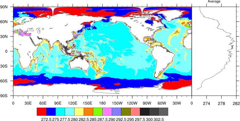
The gsn_attach_plots code isn't working because on our end, we aren't checking for map plots as a valid plot to be attached to. This is something I need to fix.
Even when I fixed this, the plot didn't look great.
So, I decided to write my own short "attach_plots" function and add it to your code. This code makes sure the tickmark lengths and labels are the same
size, and that the XY plot is the same height, before it attaches the two codes using gsn_add_annotation.
Please see the modified version of your script and the resultant PNG file. Let me know if you have any questions.
--Mary
On Mar 17, 2012, at 3:58 AM, mark collier wrote:
> load "/home/599/mac599/marsland/all_scripts.ncl"
>
> begin
>
> ifile="thetaozavg_Omon_ACCESS1-0_piControl_r1i1p1_0390-0439_ANN_LM.nc"
>
> fh=addfile(ifile,"r")
>
> A1p0=fh->thetaozavg
>
> A1p0!0="lat"
> A1p0!1="lon"
> A1p0&lat=fh->j
> A1p0&lon=fh->i
> A1p0@lat2d=fh->lat
> A1p0@lon2d=fh->lon
>
> outp="test"
>
> wks = gsn_open_wks("ps",outp)
>
> xyres = True ; xy plot mods desired
> xyres@vpWidthF = .20 ; set width of second plot
> xyres@tmXBLabelStride = 2 ; label stride
> xyres@gsnDraw = False ; don't draw yet
> xyres@gsnFrame = False ; don't advance frame yet
> xyres@gsnCenterString = "Average" ; add title
> xyres@txFontHeightF = .025 ; change font height
>
> attachres1 = True
> attachres1@gsnAttachPlotXAxis=True
> attachres2 = True
>
> res = True
> res@gsnDraw = False ; don't draw
> res@gsnFrame = False ; don't advance frame
> res@cnFillOn = True ; turn on color
> res@cnLinesOn = False
> res@gsnSpreadColors = True ; spread out color table
> res@cnLineLabelDensityF = 0.0 ; <1.0 = less, >1.0 = more
> res@cnLineLabelsOn = False
> res@cnFillMode = "AreaFill"
> res@mpCenterLonF = 180.
> res@mpMinLonF = 0.
> res@mpMaxLonF = 360.
> res@mpMinLatF = -90.0
> res@mpMaxLatF = 90.0
> res@mpFillOn = False ; turn off modern continents
>
> res@gsnAddCyclic = False
> res@gsnRightString = ""
> res@cnLevelSelectionMode = "ExplicitLevels"
>
> lat2D_A1p0=fh->lat
> lat_A1p0=lat2D_A1p0(:,0)
> lat_A1p0(245:299)=lat2D_A1p0(245:299,89);89/90 maximum latitude (base 0)
>
> plot = gsn_csm_contour_map_ce(wks,A1p0,res)
> xyp=gsn_csm_xy(wks,dim_avg(A1p0),lat_A1p0,xyres)
> attachid3=gsn_attach_plots(plot,xyp,attachres1,attachres2)
>
> resP=True
>
> gsn_panel(wks,(/plot/),(/1,1/),resP) ; now draw as one plot
>
> print("Finished "+outp+".")
>
> end
_______________________________________________
ncl-talk mailing list
List instructions, subscriber options, unsubscribe:
http://mailman.ucar.edu/mailman/listinfo/ncl-talk
- application/octet-stream attachment: xyplot.mod.ncl