Date: Tue Mar 27 2012 - 08:16:09 MDT
Hi Dave,
I saved Fanny's files and was able to reproduce the results.
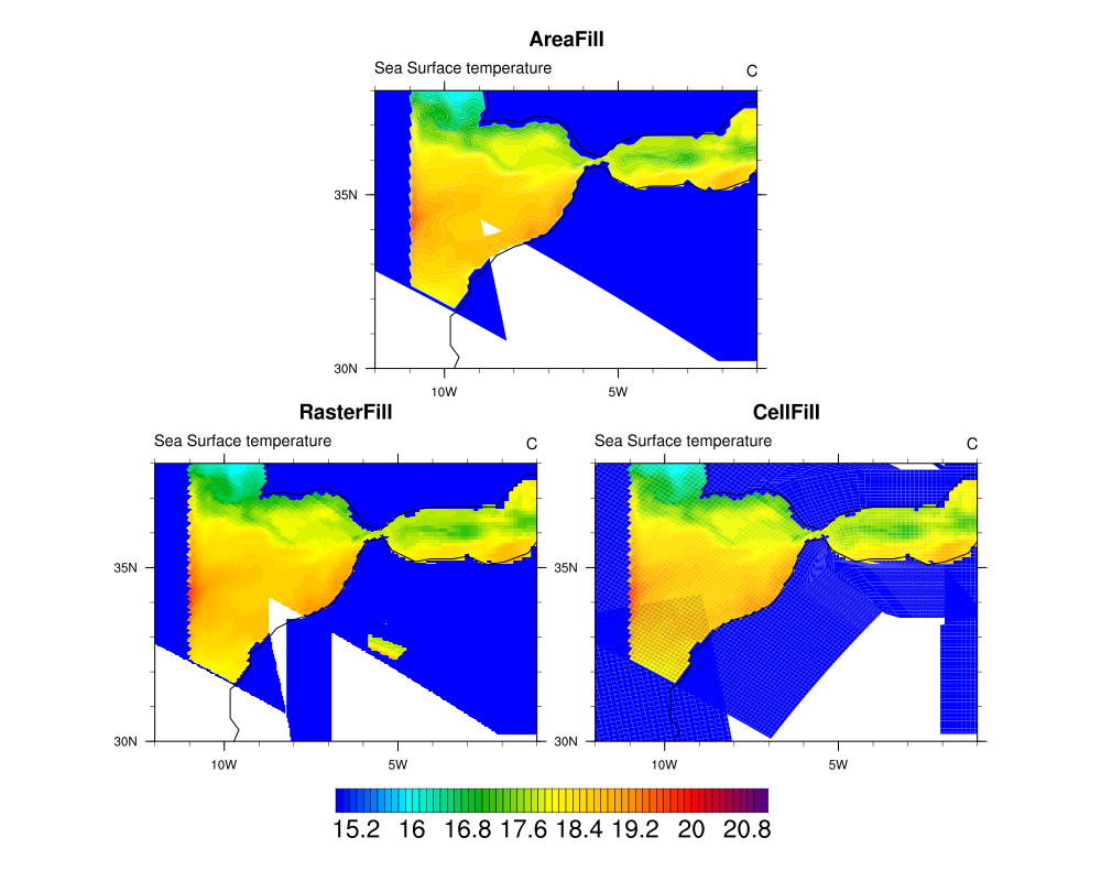
I modified her script to draw all three styles of plots (raster, area, cell) in a panel,
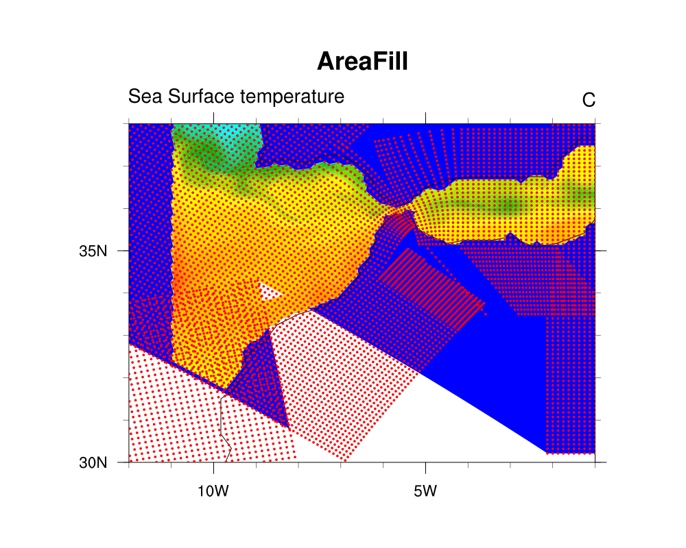
and then I added a new frame that calls gsn_draw_coordinates to draw the
lat2d/lon2d coordinates on the map as red markers.
The raster fill is rather slow, so this might be another good test for your new algorithm.
Note that the cell fill seems to produce the best plot.
I filed a ticket on this (NCL-1376) just in case.
--Mary
Begin forwarded message:
> From: "fanny.adloff" <fanny.adloff@zmaw.de>
> Subject: problem with grid from ocean model NEMOMED8
> Date: March 27, 2012 2:02:53 AM MDT
> To: <ncl-talk@ucar.edu>
>
> Dear NCL-users and developers,
>
> I have a problem to plot a simple 2D temperature field with the grid of the ocean model NEMOMED8 (Arakawa C-grid), which covers the Mediterranean Sea and a buffer zone including the near Atlantic ocean, west from Gibraltar. The grid is tilted and streched at the Gibraltar Strait, which leads to a deformation.
> I send you the NCL script and the netcdf file.
>
> I obtain a white triangle in the region around 34° LAT and -9/-8° LON.
> I don't have this problem by using a normal Contour (not a contour map).
> And I also get quite differents plots when I use AreaFill or CellFill or RasterFill.
>
> I hope that someone can help me to find a solution.
>
> Thanks by advance!
>
> Best regards,
>
> Fanny
load "$NCARG_ROOT/lib/ncarg/nclscripts/csm/gsn_code.ncl"
load "$NCARG_ROOT/lib/ncarg/nclscripts/csm/gsn_csm.ncl"
load "$NCARG_ROOT/lib/ncarg/nclscripts/csm/contributed.ncl"
begin
;=================================================
;=========== Creating a function ==============
;=================================================
undef("fannyMeta")
function fannyMeta(med:file,vName:string,lat2d[*][*],lon2d[*][*])
begin
x = med->$vName$(0,:,:)
printVarSummary(lat2d)
x@lon2d = lon2d
x@lat2d = lat2d
return (x)
end
;=================================================
;=================================================
;=================================================
;******** OPEN GRAPHICS WORKSTATION *******
wks=gsn_open_wks("pdf","temp") ;open the working session
gsn_define_colormap(wks,"BlAqGrYeOrReVi200") ;define a color palette
;********** CALLING IN DATA **********
med=addfile("NM8-24_med_1d_201112_2D_temp.nc","r")
printVarSummary(med)
;********** CONFORMING THE COORDINATES UNIT TO UNIDATA CONVENTION **********
latitude=med->nav_lat ; Making variable 2D
latitude@units = "degrees_north"
longitude=med->nav_lon ; Making variable 2D
longitude@units = "degrees_east"
; printMinMax(longitude, True)
; longitude = where(longitude.gt.180, longitude -360, longitude) ;flip the latitude >180 to negative
; printMinMax(longitude, True)
;********** ASSIGN A VARIABLE **********
SST = fannyMeta(med, "sosstsst", latitude, longitude)
printVarSummary(SST)
;********** SETTING THE RESOURCES **********
res=True
res@lbOrientation = "Horizontal"
res@gsnMaximize = True
res@cnFillOn = True
res@gsnSpreadColors = True
res@tmXBTickSpacingF = 5
res@tmYBTickSpacingF = 5
res@cnLinesOn = False ; no contour lines
res@gsnSpreadColorStart = 2
res@gsnSpreadColorEnd = 201
res@cnLabelBarEndStyle = "ExcludeOuterBoxes"
res@lbLabelAutoStride = True
res@cnLevelSelectionMode="ManualLevels"
res@cnMinLevelValF = 15
res@cnMaxLevelValF = 21
res@cnLevelSpacingF = 0.1
;************ TWO WAY TO DEFINE THE MAP REGIONS *******
res@mpMinLatF = 30 ; range to zoom in on
res@mpMaxLatF = 38
res@mpMinLonF = -12
res@mpMaxLonF = -1
res@mpGeophysicalLineThicknessF = 2
res@mpGeophysicalLineColor = 1
res@mpLandFillColor = -1
;********** PLOTTING **********CE
plot=gsn_csm_contour_map(wks,SST,res)
;=================================================
end
> _______________________________________________
> ncl-talk mailing list
> List instructions, subscriber options, unsubscribe:
> http://mailman.ucar.edu/mailman/listinfo/ncl-talk
- application/octet-stream attachment: contourmap_temp_nemo.ncl
- application/octet-stream attachment: NM8-24_med_1d_201112_2D_temp.nc