Date: Sun Aug 25 2013 - 12:05:27 MDT
Hi,
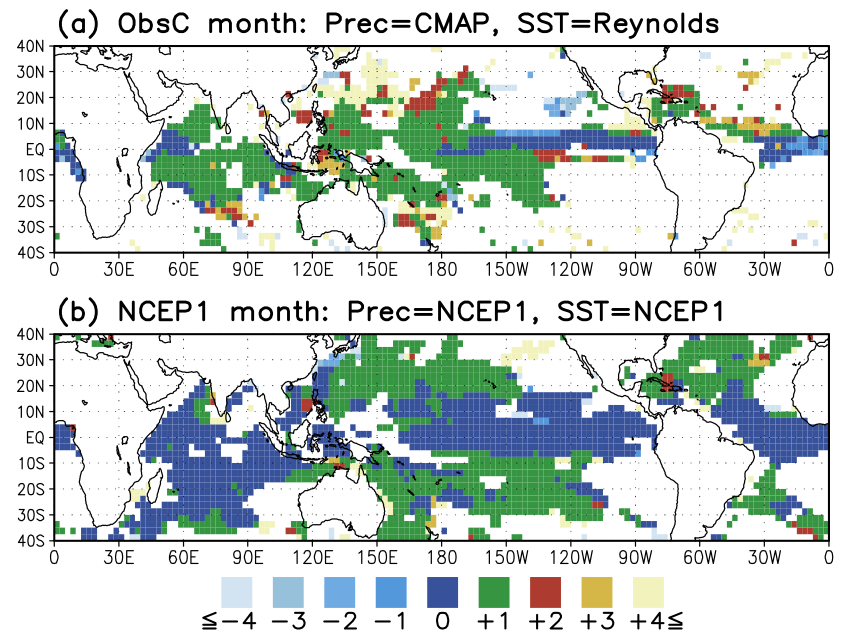
I try to plot two dimensional (lat,lon) time phase relationship between
precipitation and SST using lag correlation analysis but i had some
difficulties to create it. The plot that i want to create is very
similar to the attachedfigure from (Arakawa and Kitoh, 2004).
I created the attached NCL script to process data and calculate the
lagged correlations (in this case it is three-dimensional, lat, lon and
lags - from -30 to 30 days) and the probabilities from significance test
(using rtest function) but i need to help to convert this information to
two-dimensional plot. For specific grid cell, the data have correlations
and rtest values (i am not sure probabilities are calculated correctly
in my script) but i have to pick up the day that is in 0.01 significance
level.
You might give me some advise to create the plot from calculated statistics.
Best Regards,
--ufuk
*Ref:*
Arakawa, O., and A. Kitoh (2004), Comparison of local precipitation–SST
relationship between the observation and a reanalysis dataset, Geophys.
Res. Lett., 31, L12206, doi:10.1029/2004GL020283
;-----------------------------------------------------------
load "$NCARG_ROOT/lib/ncarg/nclscripts/csm/gsn_code.ncl"
load "$NCARG_ROOT/lib/ncarg/nclscripts/csm/gsn_csm.ncl"
load "$NCARG_ROOT/lib/ncarg/nclscripts/csm/contributed.ncl"
;-----------------------------------------------------------
begin
;--- parameters ---
yy1 = 1997
yy2 = 2000 ;2011
;--- create common time axis ---
time = yyyymmdd_time(yy1, yy2, "integer")
yyyyddd = yyyymmdd_to_yyyyddd(time)
yy = time/10000
mm = (time-(yy*10000))/100
ntime = dimsizes(time)
;--- read SST ---
ifile = "dsets/ghrsst/avhrr.oi_"+yy1+"-"+yy2+"_sub_med.nc"
ncobs1 = addfile(ifile, "r")
lsmsk = ncobs1->mask
varo1 = short2flt(ncobs1->analysed_sst)
varo1 = varo1-273.15
varo1 = mask(varo1, ismissing(varo1), False)
print(max(varo1))
dims = dimsizes(varo1)
nlat = dims(1)
nlon = dims(2)
;--- fill missing dates in SST ---
time1 = ncobs1->time
yyyymmdd1 = cd_calendar(time1, -2)
ntime1 = dimsizes(time1)
varo1_fixed = new((/ ntime, nlat, nlon /), "float")
copy_VarAtts(varo1, varo1_fixed)
do i = 0, ntime1-1
indx = ind(yyyymmdd1(i) .eq. time)
if (.not. ismissing(indx)) then
varo1_fixed(indx,:,:) = varo1(i,:,:)
end if
end do
delete(indx)
;--- read P ---
ifile = "dsets/gpcp/med/gpcpP_1997-2011_remap_day.nc"
ncobs2 = addfile(ifile, "r")
varo2 = ncobs2->precip
;--- fill missing dates in P ---
time2 = ncobs2->time
yyyymmdd2 = cd_calendar(time2, -2)
ntime2 = dimsizes(time2)
varo2_fixed = new((/ ntime, nlat, nlon /), "float")
copy_VarAtts(varo2, varo2_fixed)
do i = 0, ntime2-1
indx = ind(yyyymmdd2(i) .eq. time)
if (.not. ismissing(indx)) then
varo2_fixed(indx,:,:) = varo2(i,:,:)
end if
end do
delete(indx)
;--- apply same mask to P with SST ---
varo2_fixed = mask(varo2_fixed, ismissing(varo1_fixed), False)
;--- calculate daily anomaly of SST and P ---
varo1_day = clmDayTLL(varo1_fixed, yyyyddd)
varo1_day_ano = calcDayAnomTLL(varo1_fixed, yyyyddd, varo1_day)
delete([/ varo1, varo1_fixed, varo1_day /])
varo2_day = clmDayTLL(varo2_fixed, yyyyddd)
varo2_day_ano = calcDayAnomTLL(varo2_fixed, yyyyddd, varo2_day)
delete([/ varo2, varo2_fixed, varo2_day /])
;--- apply bandpass filter (20-100 days bandpass) to dSST and dP ---
ihp = 2
sigma = 1.0
nWgt = 201
fca = 1./100.
fcb = 1./20.
wgt = filwgts_lanczos(nWgt, ihp, fca, fcb, sigma)
varo1_day_ano_pass = wgt_runave_Wrap(varo1_day_ano(lat|:, lon|:, time|:), wgt, 0)
varo2_day_ano_pass = wgt_runave_Wrap(varo2_day_ano(lat|:, lon|:, time|:), wgt, 0)
;--- compute lead/lag correlation between dSST and dP ---
dmin = -30
dmax = 30
mxlag = dmax
times = ispan(dmin, dmax, 1)
ntimes = dimsizes(times)
corr = new((/ nlat, nlon, ntimes /), typeof(varo1_day_ano_pass))
p_lead_sst = esccr(varo2_day_ano_pass(lat|:,lon|:,time|:), \
varo1_day_ano_pass(lat|:,lon|:,time|:), mxlag)
sst_lead_p = esccr(varo1_day_ano_pass(lat|:,lon|:,time|:), \
varo2_day_ano_pass(lat|:,lon|:,time|:), mxlag)
corr(:,:,0:mxlag-1) = sst_lead_p(:,:,1:mxlag:-1)
corr(:,:,mxlag:) = p_lead_sst(:,:,0:mxlag)
copy_VarMeta(varo2_day_ano_pass(lat|:,lon|:,time|0:ntimes-1), corr)
;do i = 0, ntimes-1
; print(sprinti("%04d", times(i))+" "+\
; sprintf("%8.4f", min(corr(:,:,i)))+" "+\
; sprintf("%8.4f", max(corr(:,:,i))))
;end do
;--- significance test over correlation coefficents ---
siglvl = 0.01
prob = corr
prob = 0.0
Nr = dimsizes(varo1_day_ano_pass(0,0,:))
prob(:,:,0:mxlag-1) = rtest(corr(:,:,0:mxlag-1), Nr, 0)
prob(:,:,mxlag:) = rtest(corr(:,:,mxlag:), Nr, 0)
;do lag = 0, ntimes-1
; prob(:,:,lag) = rtest(corr(:,:,lag), Nr, 0)
; ;prob(:,:,lag) = (1.0-rtest(corr(:,:,lag), Nr, 0))*100.0
;end do
prob = mask(prob, ismissing(corr), False)
do i = 0, ntimes-1
print(sprinti("%04d", times(i))+" "+\
sprintf("%8.4f", min(prob(:,:,i)))+" "+\
sprintf("%8.4f", max(prob(:,:,i))))
end do
;********************************************************
; Actually i need to help to write this part
;********************************************************
;--- find highest correlated lag days ---
sign1 = corr(:,:,0)
sign1 = corr@_FillValue
sign2 = sign1
prob = mask(prob, prob .lt. siglvl, True)
do i = 0, nlat-1
do j = 0, nlon-1
if (any(.not. ismissing(prob(i,j,0:mxlag-1)))) then
ind1 = ind(prob(i,j,0:mxlag-1) .eq. max(prob(i,j,0:mxlag-1)))
sign1(i,j) = (/ times(ind1) /)
end if
if (any(.not. ismissing(prob(i,j,mxlag:)))) then
ind2 = ind(prob(i,j,mxlag:) .eq. max(prob(i,j,mxlag:)))
sign2(i,j) = (/ times(mxlag+ind2) /)
end if
end do
end do
copy_VarMeta(corr(lat|:,lon|:,time|0), sign1)
copy_VarMeta(corr(lat|:,lon|:,time|0), sign2)
;********************************************************
;--- plot data ---
wks = gsn_open_wks("newpdf", "plot_sst-p_lag_2d")
gsn_define_colormap(wks, "gsn_default")
i = NhlNewColor(wks, 0.8, 0.8, 0.8)
res = True
res@gsnFrame = False
res@gsnAddCyclic = False
res@gsnLeftString = ""
res@gsnRightString = ""
res@cnFillOn = True
res@cnFillMode = "CellFill"
res@cnInfoLabelOn = False
res@cnLinesOn = False
res@cnLineLabelsOn = False
res@tiXAxisString = "Longitude"
res@tiYAxisString = "Latitude"
res@tiXAxisSide = "Top"
res@pmTickMarkDisplayMode = "Always"
res@tiXAxisFontHeightF = 0.012
res@tiYAxisFontHeightF = 0.012
res@tmXTLabelFontHeightF = 0.012
res@tmYLLabelFontHeightF = 0.012
res@tmXBOn = False
res@tmYROn = False
res@tmXBLabelsOn = False
res@tmYRLabelsOn = False
res@lbLabelBarOn = True
res@lbLabelFontHeightF = 0.01
res@lbOrientation = "Vertical"
;res@pmLabelBarWidthF = 0.06
;--- region ---
minlon = -10.0
minlat = 25.0
maxlon = 48.0
maxlat = 50.0
;--- map definitions ---
res@mpDataBaseVersion = "HighRes"
res@mpProjection = "LambertConformal"
res@mpOutlineDrawOrder = "PostDraw"
res@mpGridAndLimbOn = False
onesix = (maxlon-minlon)/6.0
std1 = minlon+onesix
std2 = maxlon-onesix
print("[warning] -- one-six-rule standard parallels ("+\
sprintf("%6.2f", std1)+","+sprintf("%6.2f", std2)+") are used.")
res@mpLambertParallel1F = std1
res@mpLambertParallel2F = std2
res@mpLimitMode = "Corners"
res@mpLeftCornerLatF = minlat
res@mpLeftCornerLonF = minlon
res@mpRightCornerLatF = maxlat
res@mpRightCornerLonF = maxlon
clon = (maxlon+minlon)/2.0
res@mpLambertMeridianF = clon
print("[warning] -- default center longtitude ("+sprintf("%6.2f", clon)+") is used. ")
res@vpYF = 0.9
res@vpXF = 0.1
res@vpHeightF = 0.40
res@vpWidthF = 0.60
plot1 = gsn_csm_contour_map(wks, sign1, res)
;res@vpYF = 0.5
;res@vpXF = 0.1
;plot2 = gsn_csm_contour_map(wks, sign2, res)
frame(wks)
end
_______________________________________________
ncl-talk mailing list
List instructions, subscriber options, unsubscribe:
http://mailman.ucar.edu/mailman/listinfo/ncl-talk