Date: Thu, 25 Jan 2007 17:26:14 -0700
Adam and Steve,
Actually there is a way to preserve the speed that comes with having
tfDoNDCOverlay set to True and still zoom a pre-projected plot: subset
the data
such that it matches the boundaries of the zoomed in map. The tricky
part is figuring out how
to find the section of the data that matches. Since the coordinates
are 2D you cannot
subscript using coordinate subscripting so you need to figure out the
appropriate
subscripting indexes.
There is a relatively straightforward way to do this using
what are known as 'Normalized Projection Coordinates' in the MapPlot
object.
For any map projection the NPC values go from 0 to 1 left to right and
bottom to top
for the maximal area plot. These values are linear across the projected
area.
When the map plot space is limited by setting map limit values using
any of
the mpLimitModes the NPC limits of that space can be determined using
'getvalues'
with the resources mp[Left|Right|Top|Bottom]NPCF. Given these values
from the map
both before and after 'zooming' it, you can use simple ratios to
determine subsetting
indexes for the data.
Here is code that I added to the end of Steve's code that does the
required
calculations and does a zoomed in plot. I'm also including my modified
version as an attachment.
Note that I adjusted the file name to a RUC file I downloaded today.
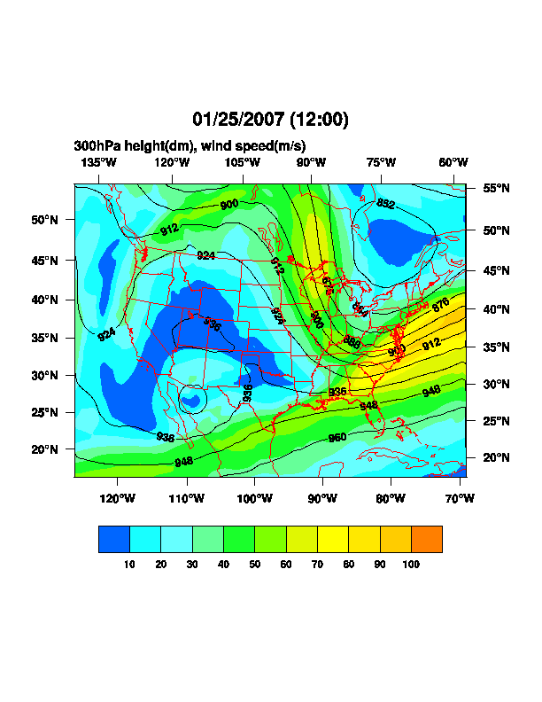
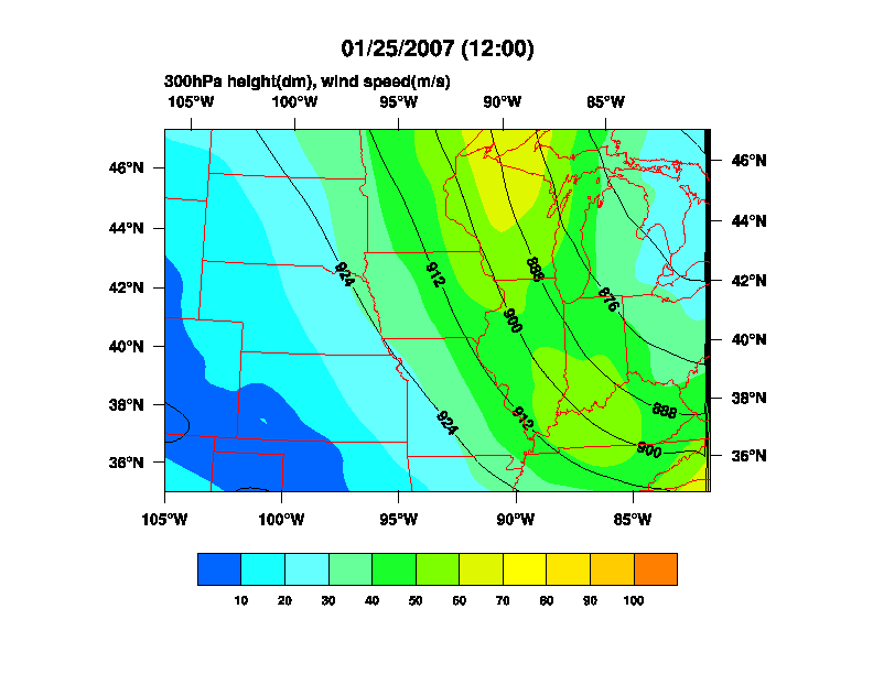
Also attached are plots that were
produced by the code. This is a little tricky but certainly faster than
using 2D coordinates to
transform the data into the map projection space. It would be nice if
we could come up
with an easier way to use the technique.
-dave
plot1 =
gsn_csm_contour_map_overlay(wks,spd(index300,:,:),z(index300,:,:)/
10.,res1,res2) ; Draw contours over a map.
; draw(plot1)
; frame(wks)
; added code:
;===================
getvalues plot1
"mpLeftNPCF" : lnpc
"mpBottomNPCF" : bnpc
"mpTopNPCF" : tnpc
"mpRightNPCF" : rnpc
end getvalues
print("NPC (before zooming) bottom: " + bnpc + " left: " + lnpc + "
top: " + tnpc + " right: " + rnpc)
res1_at_mpLeftCornerLatF = 35.
res1_at_mpLeftCornerLonF = -105.
res1_at_mpRightCornerLatF = 47.
res1_at_mpRightCornerLonF = -80.
plot1 =
gsn_csm_contour_map_overlay(wks,spd(index300,:,:),z(index300,:,:)/
10.,res1,res2) ; Draw contours over a map.
getvalues plot1
"mpLeftNPCF" : lnpc1
"mpBottomNPCF" : bnpc1
"mpTopNPCF" : tnpc1
"mpRightNPCF" : rnpc1
end getvalues
print("NPC (after zooming) bottom: " + bnpc1 + " left: " + lnpc1 + "
top: " + tnpc1 + " right: " + rnpc1)
width = rnpc - lnpc
lf = (lnpc1 - lnpc) / width
rf = (rnpc1 - lnpc) / width
height = tnpc - bnpc
bf = (bnpc1 - bnpc) / height
tf = (tnpc1 - bnpc) / height
print("Fractional distance from bottom left, left: " + lf + " right:
" + rf + " bottom: " + bf + " top: " + tf)
dims = dimsizes(spd)
xgrid = dims(2)
ygrid = dims(1)
xl = floattoint(lf * xgrid)
xr = floattoint(rf * xgrid)
yl = floattoint(bf * ygrid)
yr = floattoint(tf * ygrid)
print("Grid subscripting indexes, x left: " + xl + " x right: " + xr
+ " y left: " + yl + " yright: " + yr)
print("Coordinates at these subscripts, bottom left lat/lon: " \
+ f->gridlat_252(yl,xl) + "," + f->gridlon_252(yl,xl) + \
" top right lat/lon: " + f->gridlat_252(yr,xr) + "," +
f->gridlon_252(yr,xr))
plot1 =
gsn_csm_contour_map_overlay(wks,spd(index300,yl:yr,xl:
xr),z(index300,yl:yr,xl:xr)/10.,res1,res2) ; Draw contours over a
map.
draw(plot1)
frame(wks)
On Jan 25, 2007, at 1:37 PM, Adam Phillips wrote:
> Hello all,
>
> Steve's issue was resolved by attaching the 2D latitudes/longitudes to
> his data array, and by setting tfDoNDCOverlay = False (which is the
> default). Specifically, if the variable to be plotted is "x"
>
> x = f->FOO
> x_at_lon2d = f->XLON ; XLON is the 2d array on the file
> x_at_lat2d = f->XLAT
>
> The special attributes "lat2d" and "lon2d" are recognized
> by the gsn plotting routines.
>
> =======
>
> This example brings up a very good point. When you are dealing with two
> dimensional latitudes/longitudes, you have 2 choices when it comes to
> plotting the data:
>
> 1) set tfDoNDCOverlay = True, mpLimitMode = "Corners", and the
> mpLeftCornerLatF, mpLeftCornerLonF, mpRightCornerLatF, and
> mpRightCornerLonF resources. In terms of drawing speed this is the
> fastest way. The limitation is that you cannot zoom in onto a
> particular region. This method is faster because NCL takes the
> data passed into the plotting function and draws it in the
> region specified by the mp*Corner*F resources above. No
> map transformation computations are performed.
>
> or
>
> 2) attach the 2D lats,lons to the array. (See above and
> http://www.ncl.ucar.edu/Applications/Scripts/popscal_1.ncl).
> This method draws slightly slower than the first method
> because it computes the required map transformations.
> The advantage is that it allows the flexibility of
> zooming in onto a particular region.
>
> Adam + Dennis
>
> Steve Nesbitt wrote:
>> Hello,
>> I am trying to plot RUC model data using NCL (4.2.0.a033 on linux).
>> I can plot maps of the data over the entire domain, but when I try to
>> subset the data over the Midwest, for example (if you look carefully)
>> the map zooms in but the data does not. The attached images show
>> this behavior. See the script below for my attempt at zooming in.
>> If you want access to the raw data to try, let me know.
>> Thanks,
>> -Steve
>> ;*******************************************************
>> ; plotetaruc.ncl
>> ;*******************************************************
>> load "$NCARG_ROOT/lib/ncarg/nclscripts/csm/gsn_code.ncl" load
>> "$NCARG_ROOT/lib/ncarg/nclscripts/csm/gsn_csm.ncl" load
>> "$NCARG_ROOT/lib/ncarg/nclscripts/csm/contributed.ncl" begin
>> ;************************************************
>> ; open file and read in data
>> ;************************************************
>> diri = "./"
>> fili = "my.grb"
>> f = addfile (diri+fili, "r")
>> names = getfilevarnames(f)
>> ; print(names)
>> ; printVarSummary(names)
>> atts = getfilevaratts(f,names(0))
>> ; dims = getfilevardims(f,names(0))
>> ; print(atts)
>> ; print(dims)
>> ; get vars w = f->V_VEL_252_ISBL
>> u = f->U_GRD_252_ISBL
>> v = f->V_GRD_252_ISBL
>> z = f->HGT_252_ISBL
>> zeta = f->ABS_V_252_ISBL
>> t = f->TMP_252_ISBL
>> t_sfc = f->TMP_252_SFC
>> u_sfc = f->U_GRD_252_HTGL
>> v_sfc = f->V_GRD_252_HTGL
>> pmsl = f->MSLMA_252_MSL
>> rh = f->R_H_252_ISBL
>> spd = u*0.
>> spd = (u^2.+v^2)^0.5 prate= f->PRATE_252_SFC
>> pres = f->lv_ISBL2
>> lat2d = f->gridlat_252 lon2d = f->gridlon_252
>> time=w_at_initial_time
>> print(time)
>> ;printVarSummary(lat)
>> dims=dimsizes(w)
>> ; print(dims)
>> nlon=dims(2)
>> nlat=dims(1)
>> ; print(nlon)
>> ; print(nlat)
>> ; print(var)
>> ; print(pres(12))
>> ; printVarSummary(var)
>> ; printVarSummary(lon2d)
>> ; printVarSummary(lat2d)
>> ;*************************
>> ;common plotting resources
>> ;*************************
>> res = True ; plot mods desired
>> res_at_gsnDraw = False
>> res_at_gsnFrame = False
>> res_at_cnLinesOn = False
>> res_at_cnFillOn = True ; color plot desired
>> res_at_cnLineLabelsOn = False ; turn off contour lines
>> res_at_gsnAddCyclic = False
>> ; !!!!! any plot of data that is on a native grid, must use the
>> "corners"
>> ; method of zooming in on map.
>> ;**** ZOOMED IN
>> res_at_mpLimitMode = "Corners" ; choose range of map
>> res_at_mpLeftCornerLatF = 35.
>> res_at_mpLeftCornerLonF = -105.
>> res_at_mpRightCornerLatF = 47.
>> res_at_mpRightCornerLonF = -80.
>> ;**** ZOOMED OUT
>> res_at_mpLimitMode = "Corners" ; choose range of map
>> res_at_mpLeftCornerLatF = lat2d(0,0)
>> res_at_mpLeftCornerLonF = lon2d(0,0)
>> res_at_mpRightCornerLatF = lat2d(nlat-1,nlon-1)
>> res_at_mpRightCornerLonF = lon2d(nlat-1,nlon-1)
>> ;
>> ; The following 4 pieces of information are REQUIRED to properly
>> display
>> ; data on a native lambert conformal grid. This data should be
>> specified
>> ; somewhere in the model itself.
>> ; WARNING: our local RCM users could not provide us with this
>> information,
>> ; so this is our best guess as to the correct numbers. Use at your
>> own risk.
>> res_at_mpProjection = "LambertConformal"
>> res_at_mpLambertParallel1F = lon2d_at_Latin1
>> res_at_mpLambertParallel2F = lon2d_at_Latin2
>> res_at_mpLambertMeridianF = lon2d_at_Lov
>> ; usually, when data is placed onto a map, it is TRANSFORMED to the
>> specified
>> ; projection. Since this model is already on a native lambert
>> conformal grid,
>> ; we want to turn OFF the tranformation.
>> res_at_tfDoNDCOverlay = True
>> res_at_mpGeophysicalLineColor = "red" ; color of
>> continental outlines
>> res_at_mpPerimOn = True ; draw box
>> around map
>> res_at_mpGridLineDashPattern = 2 ; lat/lon
>> lines as dashed
>> res_at_mpOutlineBoundarySets = "GeophysicalAndUSStates" ; add state
>> boundaries
>> res_at_mpUSStateLineColor = "red" ; make them
>> red
>> res_at_pmTickMarkDisplayMode = "Always" ; turn on
>> tickmarks
>> res_at_cnLineLabelInterval = 1
>> res_at_cnLabelMasking = True
>> res_at_gsnSpreadColors=True
>> res_at_gsnSpreadColorStart = 3
>> res_at_gsnSpreadColorEnd = 19 wks = gsn_open_wks("ps","ruc_300")
>> ; open a workstation
>> ;plot=new(4,graphic)
>> gsn_define_colormap(wks,"gui_default") ; choose colormap
>> ;************************************************
>> ; create plot: upper left
>> ;************************************************
>> res1=res
>> res1_at_tiMainString=time
>> res1_at_gsnLeftString="300hPa height(dm), wind speed(m/s) "
>> res1_at_cnLevelSelectionMode = "ManualLevels" ; manual levels
>> res1_at_cnMinLevelValF = 10. ; min level
>> res1_at_cnMaxLevelValF = 100. ; max level
>> res1_at_cnLevelSpacingF = 10 ; contour spacing
>> res2=True
>> res2_at_tfDoNDCOverlay = True
>> res2_at_cnInfoLabelOn = False
>> res2_at_cnMinLevelValF = 900.+12*12 ; set min
>> contour level
>> res2_at_cnMaxLevelValF = 900.-12*12 ; set max
>> contour level
>> res2_at_cnLevelSpacingF = 12. ; set contour spacing
>> res2_at_cnLineLabelsOn = True
>> res2_at_cnLineLabelInterval = 1
>> res2_at_cnLabelMasking = True
>> ; res2_at_cnHighLabelsOn = True; label highs
>> ; res2_at_cnHighLabelString = "H"; highs' label
>> ; res2_at_cnHighLabelFontHeightF = 0.03; larger H labels
>> ; res2_at_cnHighLabelFont = "helvetica-bold"; H labels font
>> ; res2_at_cnHighLabelBackgroundColor = "Transparent"; no box
>> ; res2_at_cnLowLabelsOn = True; label lows
>> ; res2_at_cnLowLabelString = "L"; lows' label
>> ; res2_at_cnLowLabelFontHeightF = 0.03; larger L labels
>> ; res2_at_cnLowLabelFont = "helvetica-bold"; L labels font
>> ; res2_at_cnLowLabelBackgroundColor = "Transparent"; no box
>> ; res2_at_cnConpackParams = (/ "HLX:6, HLY:6" /)
>> index300=ind(pres.eq.300.)
>> plot1 =
>> gsn_csm_contour_map_overlay(wks,spd(index300,:,:),z(index300,:,:)/
>> 10.,res1,res2) ; Draw contours over a map.
>> draw(plot1)
>> frame(wks)
>> ----------------------------------------------------------------------
>> --
>> _______________________________________________
>> ncl-talk mailing list
>> ncl-talk_at_ucar.edu
>> http://mailman.ucar.edu/mailman/listinfo/ncl-talk
>
> --
> --------------------------------------------------------------
> Adam Phillips asphilli_at_ucar.edu
> National Center for Atmospheric Research tel: (303) 497-1726
> ESSL/CGD/CAS fax: (303) 497-1333
> P.O. Box 3000
> Boulder, CO 80307-3000 http://www.cgd.ucar.edu/cas/asphilli
> _______________________________________________
> ncl-talk mailing list
> ncl-talk_at_ucar.edu
> http://mailman.ucar.edu/mailman/listinfo/ncl-talk
_______________________________________________
ncl-talk mailing list
ncl-talk_at_ucar.edu
http://mailman.ucar.edu/mailman/listinfo/ncl-talk