Date: Tue Jun 26 2012 - 08:37:31 MDT
I really stump here. Surprise why my code did not work.
Need help for expert please
Mark
On Mon, Jun 25, 2012 at 7:27 PM, mark vogel <mdvogelii@gmail.com> wrote:
> Dear all
> I already added
>
> lat2d@units = "degrees_north"
> lon2d@units = "degrees_east"
> xavg@lat2d = lat2d
> xavg@lon2d = lon2d
>
>
> in my code file but I still got the same results.
> The values are all lesser than -30 while in the text file, there are
> values > 100.
> I defined 1e-33 as the fill_value.
> What have I done wrong?
> Thanks
> Mark
>
> On Mon, Jun 25, 2012 at 6:52 PM, David Brown <dbrown@ucar.edu> wrote:
>
>> Hi Mark,
>>
>> You have the lines:
>>
>> x@lat2d = lat2d
>> x@lon2d = lon2d
>> y@lat2d = lat2d
>> y@lon2d = lon2d
>>
>>
>> Have you added similar code for xavg and yavg? Note that these are not
>> coordinate variables (because 2D coordinate variables are not supported).
>> They are attributes.
>> You would be better off doing:
>> lat2d@units = "degrees_north"
>> lon2d@units = "degrees_east"
>> xavg@lat2d = lat2d
>> xavg@lon2d = lon2d
>>
>> etc.
>> -dave
>>
>>
>>
>> On Jun 25, 2012, at 4:30 PM, mark vogel wrote:
>>
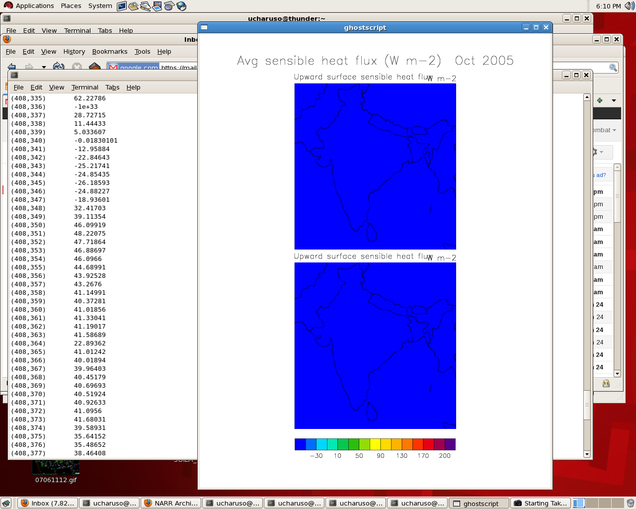
>> Dear Ncl-talk
>> I try to plot the average out. The values look ok but the plot give me
>> very low values (blue color in screenshot)
>> I add xavg and yavg average in there but I am not sure what unit is.
>> What a unit I should put it in? I put xavg&lat2d@unit = "degree_north"
>> I got the error that said
>> fatal:(lat2d) is not a named dimension in variable (xavg).
>> fatal:Execute: Error occurred at or near line 64 in file hfx_nov2.ncl
>>
>> After I comment it and I still get this error message.
>> (0) check_for_y_lat_coord: Warning: Data either does not contain a
>> valid latitude coordinate array or doesn't contain one at all.
>> (0) A valid latitude coordinate array should have a 'units' attribute
>> equal to one of the following values:
>> (0) 'degrees_north' 'degrees-north' 'degree_north' 'degrees
>> north' 'degrees_N' 'Degrees_north' 'degree_N' 'degreeN' 'degreesN' 'deg
>> north'
>> (0) check_for_lon_coord: Warning: Data either does not contain a
>> valid longitude coordinate array or doesn't contain one at all.
>> (0) A valid longitude coordinate array should have a 'units'
>> attribute equal to one of the following values:
>> (0) 'degrees_east' 'degrees-east' 'degree_east' 'degrees east'
>> 'degrees_E' 'Degrees_east' 'degree_E' 'degreeE' 'degreesE' 'deg east'
>>
>>
>> On Wed, Jun 13, 2012 at 1:22 PM, David Brown <dbrown@ucar.edu> wrote:
>>
>>> Hi Mark,
>>> You are adding the coordinate variables to x and y, but you are plotting
>>> xavg and yavg. You need to add the coordinate variables to xavg and yavg.
>>> Also check the coordinate variables
>>> to make sure they have units that match what the warning messages say
>>> they should be.
>>> -dave
>>>
>>>
>>> On Jun 13, 2012, at 10:52 AM, mark vogel wrote:
>>>
>>> Dear All
>>>
>>> I still can not generate the plot for my code, the average look correct
>>> but when I averaged it, it has an error message about coordinate. I think I
>>> specific something wrong in graphic part but could not find what is it.
>>> Please help me.
>>>
>>> (0) check_for_y_lat_coord: Warning: Data either does not contain a
>>> valid latitude coordinate array or doesn't contain one at all.
>>> (0) A valid latitude coordinate array should have a 'units'
>>> attribute equal to one of the following values:
>>> (0) 'degrees_north' 'degrees-north' 'degree_north' 'degrees
>>> north' 'degrees_N' 'Degrees_north' 'degree_N' 'degreeN' 'degreesN' 'deg
>>> north'
>>> (0) check_for_lon_coord: Warning: Data either does not contain a
>>> valid longitude coordinate array or doesn't contain one at all.
>>> (0) A valid longitude coordinate array should have a 'units'
>>> attribute equal to one of the following values:
>>> (0) 'degrees_east' 'degrees-east' 'degree_east' 'degrees east'
>>> 'degrees_E' 'Degrees_east' 'degree_E' 'degreeE' 'degreesE' 'deg east'
>>>
>>>
>>> The code is below
>>>
>>> xavg = dim_avg_n(x1,0)
>>> yavg = dim_avg_n(y1,0)
>>> xavg@units = " (a) (Default)"
>>> yavg@units = " (b) (GEM)"
>>> printVarSummary(yavg)
>>> printVarSummary(xavg)
>>> x@lat2d = lat2d
>>> x@lon2d = lon2d
>>> y@lat2d = lat2d
>>> y@lon2d = lon2d
>>>
>>>
>>> ;************************************************
>>> ; The file should be examined via: ncdump -v grid_type static.wrsi
>>> ; This will print the print type. then enter below.
>>> ;************************************************
>>> projection = "LambertConformal"
>>> ;************************************************
>>> ; create plots
>>> ;************************************************
>>> wks = gsn_open_wks("ps" ,"sh_Nov2005avg_noon") ;
>>> ps,pdf,x11,ncgm,eps
>>> gsn_define_colormap(wks ,"BlAqGrYeOrReVi200"); choose colormap
>>>
>>> res = True ; plot mods desired
>>> res@gsnSpreadColors = True ; use full range of
>>> colormap
>>> res@cnFillOn = True ; color plot desired
>>> ; res@mpMinLonF = -120 ; set min lon
>>> ; res@mpMaxLonF = -85 ; set max lon
>>> ; res@mpMinLatF = 30. ; set min lat
>>> res@vpWidthF = 0.9 ; height and width of plot
>>> res@vpHeightF = 0.4
>>>
>>> res@cnLinesOn = False ; turn off contour lines
>>> res@cnLineLabelsOn = False ; turn off contour labels
>>> res@lbLabelBarOn = False ; turn off individual
>>> lb's
>>> res@cnFillMode = "RasterFill" ; activate raster mode
>>> res@cnLevelSelectionMode = "ManualLevels" ; set manual contour
>>> levels
>>> res@cnMinLevelValF = -50 ; set min contour level
>>> res@cnMaxLevelValF = 200 ; set max contour level
>>> res@cnLevelSpacingF = 20 ; set contour spacing
>>> ;************************************************
>>> projection = "Mercator"
>>> ; projection = "LambertConformal"
>>>
>>>
>>> dimll = dimsizes(lat2d)
>>> nlat = dimll(0)
>>> mlon = dimll(1)
>>>
>>>
>>> res@mpProjection = projection
>>> res@mpLimitMode = "Corners"
>>> res@mpLeftCornerLatF = lat2d(0,0)
>>> res@mpLeftCornerLonF = lon2d(0,0)
>>> res@mpRightCornerLatF = lat2d(nlat-1,mlon-1)
>>> res@mpRightCornerLonF = lon2d(nlat-1,mlon-1)
>>>
>>> res@mpCenterLonF = 81.45 ; set center logitude
>>>
>>> if (projection.eq."LambertConformal") then
>>> res@mpLambertParallel1F = 30
>>> res@mpLambertParallel2F = 60
>>> res@mpLambertMeridianF = -90
>>> end if
>>>
>>> res@mpFillOn = False ; turn off map fill
>>> res@mpOutlineDrawOrder = "PostDraw" ; draw continental
>>> outline last
>>> res@mpOutlineBoundarySets = "National" ; state boundaries
>>>
>>> res@tfDoNDCOverlay = False ; True for 'native' grid
>>> res@gsnAddCyclic = False ; data are not cyclic
>>> ; res@lbOrientation = "vertical"
>>>
>>> ;************************************************
>>> ; allocate array for 3 plots
>>> ;************************************************
>>> plts = new (2,"graphic")
>>>
>>> ;************************************************
>>> ; Tell NCL not to draw or advance frame for individual plots
>>> res@gsnDraw = False ; (a) do not draw
>>> res@gsnFrame = False ; (b) do not advance
>>> 'frame'
>>>
>>> plts(0) = gsn_csm_contour_map(wks,xavg(:,:),res)
>>> plts(1) = gsn_csm_contour_map(wks,yavg(:,:),res)
>>> ;************************************************
>>> ; create panel: panel plots have their own set of resources
>>> ;************************************************
>>> resP = True ; modify the panel plot
>>> resP@txString = "Avg sensible heat flux (W m-2) Nov 2005"
>>> resP@gsnMaximize = True ; maximize panel area
>>> resP@gsnPanelLabelBar = True ; add common colorbar
>>> resP@lbLabelAutoStride= True ; let NCL figure lb
>>> stride
>>> resP@gsnPanelRowSpec = True ; specify 1 top, 2
>>> lower level
>>> gsn_panel(wks,plts,(/1,2/),resP) ; now draw as one plot
>>>
>>> end
>>>
>>>
>>>
>>> On Tue, Jun 12, 2012 at 5:03 PM, David Brown <dbrown@ucar.edu> wrote:
>>>
>>>> Mark,
>>>> If your data is hourly and you want to start at the same time every
>>>> day, the stride value should be 24. In other words,
>>>>
>>>> do n = 5, ntim, 24
>>>> ; ... n will be positioned at the first hour you want
>>>> end do
>>>>
>>>> On Jun 12, 2012, at 2:05 PM, mark vogel wrote:
>>>>
>>>> Dear Ncl _talk
>>>>
>>>> I did the average during afternoon time for latent heat flux as the
>>>> following code.
>>>> But when I plot it out the values are lesser than -30
>>>>
>>>> It does not seem right to me.
>>>> Anyone can help me what wrong with my code.
>>>> Thanks
>>>>
>>>> dirs = "/usr/rmt_share/tgdata/hrldas/workspace/jam2/india_out/"
>>>> ; change directory
>>>> filesn = systemfunc("ls " + dirs + "200511*LDASOUT*.nc")
>>>> filesn1 = systemfunc("ls " + dirs + "2006*LDASOUT*.nc")
>>>> f = addfiles(filesn, "r") ; change to filesn1 if 2006 )
>>>> x = f[:]->HFX(:,:,:) ; (Time,
>>>> south_north, west_east)
>>>> dirk =
>>>> "/usr/rmt_share/tgdata/hrldas/workspace/jam2/india_gemout/"
>>>> filesk = systemfunc("ls " + dirk + "200511*LDASOUT*.nc")
>>>> filesk1 = systemfunc("ls " + dirs + "2006*LDASOUT*.nc")
>>>>
>>>> g = addfiles(filesk, "r")
>>>> y = g[:]->HFX(:,:,:)
>>>> ntim = 700
>>>> nStrt = 5
>>>> nJump = 3
>>>> nSkip = 23
>>>>
>>>> do n = 5,ntim,nSkip
>>>> n1 = n
>>>> n2 = n1+nJump
>>>> print("n1="+n1+" n2="+n2)
>>>> x1 = x(n1:n2,:,:)
>>>> y1 = y(n1:n2,:,:)
>>>> xavg = dim_avg_n(x1,0)
>>>> yavg = dim_avg_n(y1,0)
>>>> end do
>>>> xavg@units = " (a) (Default)"
>>>> yavg@units = " (b) (GEM)"
>>>> printVarSummary(yavg)
>>>> printVarSummary(xavg)
>>>>
>>>> x@lat2d = lat2d
>>>> x@lon2d = lon2d
>>>> y@lat2d = lat2d
>>>> y@lon2d = lon2d
>>>>
>>>>
>>>> ;************************************************
>>>> ; The file should be examined via: ncdump -v grid_type static.wrsi
>>>> ; This will print the print type. then enter below.
>>>> ;************************************************
>>>> projection = "LambertConformal"
>>>> ;************************************************
>>>> ; create plots
>>>> ;************************************************
>>>> wks = gsn_open_wks("ps" ,"sh_Nov2005avg_noon") ;
>>>> ps,pdf,x11,ncgm,eps
>>>> gsn_define_colormap(wks ,"BlAqGrYeOrReVi200"); choose colormap
>>>>
>>>> res = True ; plot mods desired
>>>> res@gsnSpreadColors = True ; use full range of
>>>> colormap
>>>> res@cnFillOn = True ; color plot desired
>>>> ; res@mpMinLonF = -120 ; set min lon
>>>> ; res@mpMaxLonF = -85 ; set max lon
>>>> ; res@mpMinLatF = 30. ; set min lat
>>>> res@vpWidthF = 0.9 ; height and width of plot
>>>> res@vpHeightF = 0.4
>>>>
>>>> res@cnLinesOn = False ; turn off contour lines
>>>> res@cnLineLabelsOn = False ; turn off contour
>>>> labels
>>>> res@lbLabelBarOn = False ; turn off individual
>>>> lb's
>>>> res@cnFillMode = "RasterFill" ; activate raster mode
>>>> res@cnLevelSelectionMode = "ManualLevels" ; set manual contour
>>>> levels
>>>> res@cnMinLevelValF = -50 ; set min contour
>>>> level
>>>> res@cnMaxLevelValF = 200 ; set max contour level
>>>> res@cnLevelSpacingF = 20 ; set contour spacing
>>>> ;************************************************
>>>> projection = "Mercator"
>>>> res@mpProjection = projection
>>>> res@mpLimitMode = "Corners"
>>>> res@mpLeftCornerLatF = lat2d(0,0)
>>>> res@mpLeftCornerLonF = lon2d(0,0)
>>>> res@mpRightCornerLatF = lat2d(nlat-1,mlon-1)
>>>> res@mpRightCornerLonF = lon2d(nlat-1,mlon-1)
>>>>
>>>> res@mpCenterLonF = 81.45 ; set center logitude
>>>>
>>>> if (projection.eq."LambertConformal") then
>>>> res@mpLambertParallel1F = 30
>>>> res@mpLambertParallel2F = 60
>>>> res@mpLambertMeridianF = -90
>>>> end if
>>>>
>>>>
>>>>
>>>>
>>>>
>>>> res@mpFillOn = False ; turn off map fill
>>>> res@mpOutlineDrawOrder = "PostDraw" ; draw continental
>>>> outline last
>>>> res@mpOutlineBoundarySets = "National" ; state boundaries
>>>>
>>>> res@tfDoNDCOverlay = False ; True for 'native'
>>>> grid
>>>> res@gsnAddCyclic = False ; data are not cyclic
>>>> ; res@lbOrientation = "vertical"
>>>>
>>>> ;************************************************
>>>> ; allocate array for 3 plots
>>>> ;************************************************
>>>> plts = new (2,"graphic")
>>>>
>>>> ;************************************************
>>>> ; Tell NCL not to draw or advance frame for individual plots
>>>> ;************************************************
>>>> res@gsnDraw = False ; (a) do not draw
>>>> res@gsnFrame = False ; (b) do not advance
>>>> 'frame'
>>>>
>>>> plts(0) = gsn_csm_contour_map(wks,xavg(:,:),res)
>>>> plts(1) = gsn_csm_contour_map(wks,yavg(:,:),res)
>>>> ;************************************************
>>>> ; create panel: panel plots have their own set of resources
>>>> ;************************************************
>>>> resP = True ; modify the panel plot
>>>> resP@txString = "Avg sensible heat flux (W m-2) Nov 2005"
>>>> resP@gsnMaximize = True ; maximize panel area
>>>> resP@gsnPanelLabelBar = True ; add common colorbar
>>>> resP@lbLabelAutoStride= True ; let NCL figure lb
>>>> stride
>>>> resP@gsnPanelRowSpec = True ; specify 1 top, 2
>>>> lower level
>>>> gsn_panel(wks,plts,(/1,2/),resP) ; now draw as one plot
>>>>
>>>>
>>>>
>>>> On Mon, Jun 11, 2012 at 5:53 PM, Dennis Shea <shea@ucar.edu> wrote:
>>>>
>>>>> Something like
>>>>>
>>>>> ntim = dimsizes(time)
>>>>>
>>>>> nStrt = 5
>>>>> nJump = 6
>>>>> nSkip = 19
>>>>>
>>>>> do n=5,ntim-1,nSkip
>>>>> n1 = n
>>>>> n2 = n1+nJump
>>>>> print("n1="+n1+" n2="+n2)
>>>>>
>>>>> x = f->X(n1:n2,:,:)
>>>>> xavg = dim_avg_n(x,0)
>>>>> end do
>>>>>
>>>>>
>>>>> On 6/11/12 1:40 PM, mark vogel wrote:
>>>>>
>>>>>> Hi Dennis
>>>>>> I read it but I do not get it about the stride syntax.
>>>>>> I want to average the time in the afternoon for the whole month from
>>>>>> 05
>>>>>> UTC to 11 UTC
>>>>>> so I start with array 5 to arry 11 (5:11) and then want to skip 19
>>>>>> values and start again at the array 30 to 36 and then skip 19 values
>>>>>> again until the end. So I get the values only afternoon out before use
>>>>>> the dim_avg_n
>>>>>>
>>>>>> What syntax I should use?
>>>>>> Mark
>>>>>>
>>>>>> On Mon, Jun 11, 2012 at 3:24 PM, Dennis Shea <shea@ucar.edu
>>>>>> <mailto:shea@ucar.edu>> wrote:
>>>>>>
>>>>>> If you read the documentation for dim_avg,
>>>>>>
>>>>>>
>>>>>> http://www.ncl.ucar.edu/__Document/Functions/Built-in/__dim_avg.shtml<
>>>>>> http://www.ncl.ucar.edu/Document/Functions/Built-in/dim_avg.shtml>
>>>>>>
>>>>>>
>>>>>> you will see that it performs the average of the *rightmost*
>>>>>> dimension.
>>>>>>
>>>>>> (Time, south_north, west_east) ; rightmost is 'west_east'
>>>>>>
>>>>>> It is suggested that you read and use
>>>>>>
>>>>>>
>>>>>> http://www.ncl.ucar.edu/__Document/Functions/Built-in/__dim_avg_n.shtml
>>>>>>
>>>>>> <
>>>>>> http://www.ncl.ucar.edu/Document/Functions/Built-in/dim_avg_n.shtml>
>>>>>>
>>>>>> qavg = dim_avg_n(q, 0)
>>>>>> printVarSummary(qavg)
>>>>>>
>>>>>> or with meta data
>>>>>>
>>>>>>
>>>>>>
>>>>>> http://www.ncl.ucar.edu/__Document/Functions/__Contributed/dim_avg_n_Wrap.__shtml
>>>>>>
>>>>>> <
>>>>>> http://www.ncl.ucar.edu/Document/Functions/Contributed/dim_avg_n_Wrap.shtml
>>>>>> >
>>>>>>
>>>>>> qavg = dim_avg_n_Wrap(q, 0)
>>>>>> printVarSummary(qavg)
>>>>>>
>>>>>> --
>>>>>> Also, this does not look correct
>>>>>>
>>>>>>
>>>>>> f = addfiles(filesn, "r") ; change to filesn1 if 2006 )
>>>>>> x = f[:]->HFX(:,:,:) ;
>>>>>> (Time, south_north, west_east)
>>>>>> x1 = x(5:10:19,:,:)
>>>>>>
>>>>>> The 5:10:19 makes no sense. It 'say' to use index values 5 thru 10
>>>>>> in strides of 19.
>>>>>>
>>>>>> Please read about subscripting at:
>>>>>>
>>>>>>
>>>>>>
>>>>>> http://www.ncl.ucar.edu/__Document/Manuals/Ref_Manual/__NclVariables.shtml#Subscripts
>>>>>>
>>>>>> <
>>>>>> http://www.ncl.ucar.edu/Document/Manuals/Ref_Manual/NclVariables.shtml#Subscripts
>>>>>> >
>>>>>>
>>>>>>
>>>>>>
>>>>>>
>>>>>>
>>>>>> On 6/11/12 1:02 PM, mark vogel wrote:
>>>>>>
>>>>>> Hi all
>>>>>> I used dim avg to do the average for the afternoon time for
>>>>>> each
>>>>>> lat lon.
>>>>>> But I am not sure dim-avg is average for each grid.
>>>>>> It look like it averaged from west to east domain.
>>>>>> What should I used to average the time in each grid point?
>>>>>> Anyone answer me please
>>>>>> Mark
>>>>>> ---------- Forwarded message ----------
>>>>>> From: *mark vogel* <mdvogelii@gmail.com
>>>>>> <mailto:mdvogelii@gmail.com> <mailto:mdvogelii@gmail.com
>>>>>> <mailto:mdvogelii@gmail.com>>>
>>>>>> Date: Mon, Jun 11, 2012 at 1:43 PM
>>>>>> Subject: plot dim_avg
>>>>>> To: NCL USERS <ncl-talk@ucar.edu <mailto:ncl-talk@ucar.edu>
>>>>>> <mailto:ncl-talk@ucar.edu <mailto:ncl-talk@ucar.edu>>>
>>>>>>
>>>>>>
>>>>>> Dear all
>>>>>> I try to average data only for daytime and plot it out.
>>>>>> After I used dim_avg, then dimesion changed from 3 to 2
>>>>>> dimension and
>>>>>> when I used
>>>>>> gsm_contour_map to plot it out.
>>>>>>
>>>>>> Please help
>>>>>> Mark
>>>>>>
>>>>>>
>>>>>>
>>>>>> filesn1 = systemfunc("ls " + dirs + "2006*LDASOUT*.nc")
>>>>>> f = addfiles(filesn, "r") ; change to filesn1 if 2006 )
>>>>>> x = f[:]->HFX(:,:,:)
>>>>>> ; (Time,
>>>>>> south_north, west_east)
>>>>>> x1 = x(5:10:19,:,:)
>>>>>> x1@units = " (a) (Default)"
>>>>>> ; print(x)
>>>>>> dirk =
>>>>>> "/usr/rmt_share/tgdata/hrldas/__workspace/jam2/india_gemout/"
>>>>>>
>>>>>> filesk = systemfunc("ls " + dirk +
>>>>>> "200511*LDASOUT*.nc")
>>>>>> filesk1 = systemfunc("ls " + dirs +
>>>>>> "2006*LDASOUT*.nc")
>>>>>>
>>>>>> g = addfiles(filesk, "r")
>>>>>> y = g[:]->HFX(:,:,:)
>>>>>> y1 = y(5:10:19,:,:)
>>>>>>
>>>>>> y1@units = " (b) (GEM)"
>>>>>> xavg = dim_avg_Wrap(x1)
>>>>>> yavg = dim_avg_Wrap(y1)
>>>>>> ; print(x1)
>>>>>> print(yavg)
>>>>>> x@lat2d = lat2d
>>>>>> x@lon2d = lon2d
>>>>>> y@lat2d = lat2d
>>>>>> y@lon2d = lon2d
>>>>>>
>>>>>>
>>>>>> res@mpFillOn = False ; turn off
>>>>>> map fill
>>>>>> res@mpOutlineDrawOrder = "PostDraw" ; draw
>>>>>> continental
>>>>>> outline last
>>>>>> res@mpOutlineBoundarySets = "National" ; state boundaries
>>>>>>
>>>>>> res@tfDoNDCOverlay = False ; True for
>>>>>> 'native' grid
>>>>>> res@gsnAddCyclic = False ; data are not
>>>>>> cyclic
>>>>>> ; res@lbOrientation = "vertical"
>>>>>>
>>>>>> ;*****************************__*******************
>>>>>>
>>>>>> ; allocate array for 3 plots
>>>>>> ;*****************************__*******************
>>>>>>
>>>>>> plts = new (2,"graphic")
>>>>>>
>>>>>> ;*****************************__*******************
>>>>>>
>>>>>> ; Tell NCL not to draw or advance frame for individual plots
>>>>>> ;*****************************__*******************
>>>>>>
>>>>>> res@gsnDraw = False ; (a) do not
>>>>>> draw
>>>>>> res@gsnFrame = False ; (b) do not
>>>>>> advance 'frame'
>>>>>>
>>>>>> plts(0) =
>>>>>> gsn_csm_contour_map(wks,xavg(:__,:),res)
>>>>>> plts(1) =
>>>>>> gsn_csm_contour_map(wks,yavg(:__,:),res)
>>>>>> ;*****************************__*******************
>>>>>>
>>>>>>
>>>>>>
>>>>>>
>>>>>>
>>>>>> _________________________________________________
>>>>>>
>>>>>> ncl-talk mailing list
>>>>>> List instructions, subscriber options, unsubscribe:
>>>>>> http://mailman.ucar.edu/__mailman/listinfo/ncl-talk
>>>>>> <http://mailman.ucar.edu/mailman/listinfo/ncl-talk>
>>>>>>
>>>>>>
>>>>>>
>>>> _______________________________________________
>>>> ncl-talk mailing list
>>>> List instructions, subscriber options, unsubscribe:
>>>> http://mailman.ucar.edu/mailman/listinfo/ncl-talk
>>>>
>>>>
>>>>
>>>
>>>
>>> On Tue, Jun 12, 2012 at 5:03 PM, David Brown <dbrown@ucar.edu> wrote:
>>>
>>>> Mark,
>>>> If your data is hourly and you want to start at the same time every
>>>> day, the stride value should be 24. In other words,
>>>>
>>>> do n = 5, ntim, 24
>>>> ; ... n will be positioned at the first hour you want
>>>> end do
>>>>
>>>> On Jun 12, 2012, at 2:05 PM, mark vogel wrote:
>>>>
>>>> Dear Ncl _talk
>>>>
>>>> I did the average during afternoon time for latent heat flux as the
>>>> following code.
>>>> But when I plot it out the values are lesser than -30
>>>>
>>>> It does not seem right to me.
>>>> Anyone can help me what wrong with my code.
>>>> Thanks
>>>>
>>>> dirs = "/usr/rmt_share/tgdata/hrldas/workspace/jam2/india_out/"
>>>> ; change directory
>>>> filesn = systemfunc("ls " + dirs + "200511*LDASOUT*.nc")
>>>> filesn1 = systemfunc("ls " + dirs + "2006*LDASOUT*.nc")
>>>> f = addfiles(filesn, "r") ; change to filesn1 if 2006 )
>>>> x = f[:]->HFX(:,:,:) ; (Time,
>>>> south_north, west_east)
>>>> dirk =
>>>> "/usr/rmt_share/tgdata/hrldas/workspace/jam2/india_gemout/"
>>>> filesk = systemfunc("ls " + dirk + "200511*LDASOUT*.nc")
>>>> filesk1 = systemfunc("ls " + dirs + "2006*LDASOUT*.nc")
>>>>
>>>> g = addfiles(filesk, "r")
>>>> y = g[:]->HFX(:,:,:)
>>>> ntim = 700
>>>> nStrt = 5
>>>> nJump = 3
>>>> nSkip = 23
>>>>
>>>> do n = 5,ntim,nSkip
>>>> n1 = n
>>>> n2 = n1+nJump
>>>> print("n1="+n1+" n2="+n2)
>>>> x1 = x(n1:n2,:,:)
>>>> y1 = y(n1:n2,:,:)
>>>> xavg = dim_avg_n(x1,0)
>>>> yavg = dim_avg_n(y1,0)
>>>> end do
>>>> xavg@units = " (a) (Default)"
>>>> yavg@units = " (b) (GEM)"
>>>> printVarSummary(yavg)
>>>> printVarSummary(xavg)
>>>>
>>>> x@lat2d = lat2d
>>>> x@lon2d = lon2d
>>>> y@lat2d = lat2d
>>>> y@lon2d = lon2d
>>>>
>>>>
>>>> ;************************************************
>>>> ; The file should be examined via: ncdump -v grid_type static.wrsi
>>>> ; This will print the print type. then enter below.
>>>> ;************************************************
>>>> projection = "LambertConformal"
>>>> ;************************************************
>>>> ; create plots
>>>> ;************************************************
>>>> wks = gsn_open_wks("ps" ,"sh_Nov2005avg_noon") ;
>>>> ps,pdf,x11,ncgm,eps
>>>> gsn_define_colormap(wks ,"BlAqGrYeOrReVi200"); choose colormap
>>>>
>>>> res = True ; plot mods desired
>>>> res@gsnSpreadColors = True ; use full range of
>>>> colormap
>>>> res@cnFillOn = True ; color plot desired
>>>> ; res@mpMinLonF = -120 ; set min lon
>>>> ; res@mpMaxLonF = -85 ; set max lon
>>>> ; res@mpMinLatF = 30. ; set min lat
>>>> res@vpWidthF = 0.9 ; height and width of plot
>>>> res@vpHeightF = 0.4
>>>>
>>>> res@cnLinesOn = False ; turn off contour lines
>>>> res@cnLineLabelsOn = False ; turn off contour
>>>> labels
>>>> res@lbLabelBarOn = False ; turn off individual
>>>> lb's
>>>> res@cnFillMode = "RasterFill" ; activate raster mode
>>>> res@cnLevelSelectionMode = "ManualLevels" ; set manual contour
>>>> levels
>>>> res@cnMinLevelValF = -50 ; set min contour
>>>> level
>>>> res@cnMaxLevelValF = 200 ; set max contour level
>>>> res@cnLevelSpacingF = 20 ; set contour spacing
>>>> ;************************************************
>>>> projection = "Mercator"
>>>> res@mpProjection = projection
>>>> res@mpLimitMode = "Corners"
>>>> res@mpLeftCornerLatF = lat2d(0,0)
>>>> res@mpLeftCornerLonF = lon2d(0,0)
>>>> res@mpRightCornerLatF = lat2d(nlat-1,mlon-1)
>>>> res@mpRightCornerLonF = lon2d(nlat-1,mlon-1)
>>>>
>>>> res@mpCenterLonF = 81.45 ; set center logitude
>>>>
>>>> if (projection.eq."LambertConformal") then
>>>> res@mpLambertParallel1F = 30
>>>> res@mpLambertParallel2F = 60
>>>> res@mpLambertMeridianF = -90
>>>> end if
>>>>
>>>>
>>>>
>>>>
>>>>
>>>> res@mpFillOn = False ; turn off map fill
>>>> res@mpOutlineDrawOrder = "PostDraw" ; draw continental
>>>> outline last
>>>> res@mpOutlineBoundarySets = "National" ; state boundaries
>>>>
>>>> res@tfDoNDCOverlay = False ; True for 'native'
>>>> grid
>>>> res@gsnAddCyclic = False ; data are not cyclic
>>>> ; res@lbOrientation = "vertical"
>>>>
>>>> ;************************************************
>>>> ; allocate array for 3 plots
>>>> ;************************************************
>>>> plts = new (2,"graphic")
>>>>
>>>> ;************************************************
>>>> ; Tell NCL not to draw or advance frame for individual plots
>>>> ;************************************************
>>>> res@gsnDraw = False ; (a) do not draw
>>>> res@gsnFrame = False ; (b) do not advance
>>>> 'frame'
>>>>
>>>> plts(0) = gsn_csm_contour_map(wks,xavg(:,:),res)
>>>> plts(1) = gsn_csm_contour_map(wks,yavg(:,:),res)
>>>> ;************************************************
>>>> ; create panel: panel plots have their own set of resources
>>>> ;************************************************
>>>> resP = True ; modify the panel plot
>>>> resP@txString = "Avg sensible heat flux (W m-2) Nov 2005"
>>>> resP@gsnMaximize = True ; maximize panel area
>>>> resP@gsnPanelLabelBar = True ; add common colorbar
>>>> resP@lbLabelAutoStride= True ; let NCL figure lb
>>>> stride
>>>> resP@gsnPanelRowSpec = True ; specify 1 top, 2
>>>> lower level
>>>> gsn_panel(wks,plts,(/1,2/),resP) ; now draw as one plot
>>>>
>>>>
>>>>
>>>> On Mon, Jun 11, 2012 at 5:53 PM, Dennis Shea <shea@ucar.edu> wrote:
>>>>
>>>>> Something like
>>>>>
>>>>> ntim = dimsizes(time)
>>>>>
>>>>> nStrt = 5
>>>>> nJump = 6
>>>>> nSkip = 19
>>>>>
>>>>> do n=5,ntim-1,nSkip
>>>>> n1 = n
>>>>> n2 = n1+nJump
>>>>> print("n1="+n1+" n2="+n2)
>>>>>
>>>>> x = f->X(n1:n2,:,:)
>>>>> xavg = dim_avg_n(x,0)
>>>>> end do
>>>>>
>>>>>
>>>>> On 6/11/12 1:40 PM, mark vogel wrote:
>>>>>
>>>>>> Hi Dennis
>>>>>> I read it but I do not get it about the stride syntax.
>>>>>> I want to average the time in the afternoon for the whole month from
>>>>>> 05
>>>>>> UTC to 11 UTC
>>>>>> so I start with array 5 to arry 11 (5:11) and then want to skip 19
>>>>>> values and start again at the array 30 to 36 and then skip 19 values
>>>>>> again until the end. So I get the values only afternoon out before use
>>>>>> the dim_avg_n
>>>>>>
>>>>>> What syntax I should use?
>>>>>> Mark
>>>>>>
>>>>>> On Mon, Jun 11, 2012 at 3:24 PM, Dennis Shea <shea@ucar.edu
>>>>>> <mailto:shea@ucar.edu>> wrote:
>>>>>>
>>>>>> If you read the documentation for dim_avg,
>>>>>>
>>>>>> http://www.ncl.ucar.edu/__**Document/Functions/Built-in/__**
>>>>>> dim_avg.shtml<http://www.ncl.ucar.edu/__Document/Functions/Built-in/__dim_avg.shtml><
>>>>>> http://www.ncl.ucar.edu/**Document/Functions/Built-in/**dim_avg.shtml<http://www.ncl.ucar.edu/Document/Functions/Built-in/dim_avg.shtml>>
>>>>>>
>>>>>>
>>>>>>
>>>>>> you will see that it performs the average of the *rightmost*
>>>>>> dimension.
>>>>>>
>>>>>> (Time, south_north, west_east) ; rightmost is 'west_east'
>>>>>>
>>>>>> It is suggested that you read and use
>>>>>>
>>>>>> http://www.ncl.ucar.edu/__**Document/Functions/Built-in/__**
>>>>>> dim_avg_n.shtml<http://www.ncl.ucar.edu/__Document/Functions/Built-in/__dim_avg_n.shtml>
>>>>>>
>>>>>> <http://www.ncl.ucar.edu/**Document/Functions/Built-in/**
>>>>>> dim_avg_n.shtml<http://www.ncl.ucar.edu/Document/Functions/Built-in/dim_avg_n.shtml>
>>>>>> >
>>>>>>
>>>>>> qavg = dim_avg_n(q, 0)
>>>>>> printVarSummary(qavg)
>>>>>>
>>>>>> or with meta data
>>>>>>
>>>>>>
>>>>>> http://www.ncl.ucar.edu/__**Document/Functions/__**
>>>>>> Contributed/dim_avg_n_Wrap.__**shtml<http://www.ncl.ucar.edu/__Document/Functions/__Contributed/dim_avg_n_Wrap.__shtml>
>>>>>>
>>>>>> <http://www.ncl.ucar.edu/**Document/Functions/**
>>>>>> Contributed/dim_avg_n_Wrap.**shtml<http://www.ncl.ucar.edu/Document/Functions/Contributed/dim_avg_n_Wrap.shtml>
>>>>>> >
>>>>>>
>>>>>> qavg = dim_avg_n_Wrap(q, 0)
>>>>>> printVarSummary(qavg)
>>>>>>
>>>>>> --
>>>>>> Also, this does not look correct
>>>>>>
>>>>>>
>>>>>> f = addfiles(filesn, "r") ; change to filesn1 if 2006 )
>>>>>> x = f[:]->HFX(:,:,:) ;
>>>>>> (Time, south_north, west_east)
>>>>>> x1 = x(5:10:19,:,:)
>>>>>>
>>>>>> The 5:10:19 makes no sense. It 'say' to use index values 5 thru 10
>>>>>> in strides of 19.
>>>>>>
>>>>>> Please read about subscripting at:
>>>>>>
>>>>>>
>>>>>> http://www.ncl.ucar.edu/__**Document/Manuals/Ref_Manual/__**
>>>>>> NclVariables.shtml#Subscripts<http://www.ncl.ucar.edu/__Document/Manuals/Ref_Manual/__NclVariables.shtml#Subscripts>
>>>>>>
>>>>>> <http://www.ncl.ucar.edu/**Document/Manuals/Ref_Manual/**
>>>>>> NclVariables.shtml#Subscripts<http://www.ncl.ucar.edu/Document/Manuals/Ref_Manual/NclVariables.shtml#Subscripts>
>>>>>> >
>>>>>>
>>>>>>
>>>>>>
>>>>>>
>>>>>>
>>>>>> On 6/11/12 1:02 PM, mark vogel wrote:
>>>>>>
>>>>>> Hi all
>>>>>> I used dim avg to do the average for the afternoon time for
>>>>>> each
>>>>>> lat lon.
>>>>>> But I am not sure dim-avg is average for each grid.
>>>>>> It look like it averaged from west to east domain.
>>>>>> What should I used to average the time in each grid point?
>>>>>> Anyone answer me please
>>>>>> Mark
>>>>>> ---------- Forwarded message ----------
>>>>>> From: *mark vogel* <mdvogelii@gmail.com
>>>>>> <mailto:mdvogelii@gmail.com> <mailto:mdvogelii@gmail.com
>>>>>> <mailto:mdvogelii@gmail.com>>>
>>>>>> Date: Mon, Jun 11, 2012 at 1:43 PM
>>>>>> Subject: plot dim_avg
>>>>>> To: NCL USERS <ncl-talk@ucar.edu <mailto:ncl-talk@ucar.edu>
>>>>>> <mailto:ncl-talk@ucar.edu <mailto:ncl-talk@ucar.edu>>>
>>>>>>
>>>>>>
>>>>>> Dear all
>>>>>> I try to average data only for daytime and plot it out.
>>>>>> After I used dim_avg, then dimesion changed from 3 to 2
>>>>>> dimension and
>>>>>> when I used
>>>>>> gsm_contour_map to plot it out.
>>>>>>
>>>>>> Please help
>>>>>> Mark
>>>>>>
>>>>>>
>>>>>>
>>>>>> filesn1 = systemfunc("ls " + dirs + "2006*LDASOUT*.nc")
>>>>>> f = addfiles(filesn, "r") ; change to filesn1 if 2006 )
>>>>>> x = f[:]->HFX(:,:,:)
>>>>>> ; (Time,
>>>>>> south_north, west_east)
>>>>>> x1 = x(5:10:19,:,:)
>>>>>> x1@units = " (a) (Default)"
>>>>>> ; print(x)
>>>>>> dirk =
>>>>>> "/usr/rmt_share/tgdata/hrldas/**__workspace/jam2/india_gemout/
>>>>>> **"
>>>>>>
>>>>>> filesk = systemfunc("ls " + dirk +
>>>>>> "200511*LDASOUT*.nc")
>>>>>> filesk1 = systemfunc("ls " + dirs +
>>>>>> "2006*LDASOUT*.nc")
>>>>>>
>>>>>> g = addfiles(filesk, "r")
>>>>>> y = g[:]->HFX(:,:,:)
>>>>>> y1 = y(5:10:19,:,:)
>>>>>>
>>>>>> y1@units = " (b) (GEM)"
>>>>>> xavg = dim_avg_Wrap(x1)
>>>>>> yavg = dim_avg_Wrap(y1)
>>>>>> ; print(x1)
>>>>>> print(yavg)
>>>>>> x@lat2d = lat2d
>>>>>> x@lon2d = lon2d
>>>>>> y@lat2d = lat2d
>>>>>> y@lon2d = lon2d
>>>>>>
>>>>>>
>>>>>> res@mpFillOn = False ; turn off
>>>>>> map fill
>>>>>> res@mpOutlineDrawOrder = "PostDraw" ; draw
>>>>>> continental
>>>>>> outline last
>>>>>> res@mpOutlineBoundarySets = "National" ; state boundaries
>>>>>>
>>>>>> res@tfDoNDCOverlay = False ; True for
>>>>>> 'native' grid
>>>>>> res@gsnAddCyclic = False ; data are not
>>>>>> cyclic
>>>>>> ; res@lbOrientation = "vertical"
>>>>>>
>>>>>> ;*******************************__*******************
>>>>>>
>>>>>> ; allocate array for 3 plots
>>>>>> ;*******************************__*******************
>>>>>>
>>>>>> plts = new (2,"graphic")
>>>>>>
>>>>>> ;*******************************__*******************
>>>>>>
>>>>>> ; Tell NCL not to draw or advance frame for individual plots
>>>>>> ;*******************************__*******************
>>>>>>
>>>>>> res@gsnDraw = False ; (a) do not
>>>>>> draw
>>>>>> res@gsnFrame = False ; (b) do not
>>>>>> advance 'frame'
>>>>>>
>>>>>> plts(0) =
>>>>>> gsn_csm_contour_map(wks,xavg(:**__,:),res)
>>>>>> plts(1) =
>>>>>> gsn_csm_contour_map(wks,yavg(:**__,:),res)
>>>>>> ;*******************************__*******************
>>>>>>
>>>>>>
>>>>>>
>>>>>>
>>>>>>
>>>>>> ______________________________**___________________
>>>>>>
>>>>>> ncl-talk mailing list
>>>>>> List instructions, subscriber options, unsubscribe:
>>>>>> http://mailman.ucar.edu/__**mailman/listinfo/ncl-talk<http://mailman.ucar.edu/__mailman/listinfo/ncl-talk>
>>>>>> <http://mailman.ucar.edu/**mailman/listinfo/ncl-talk<http://mailman.ucar.edu/mailman/listinfo/ncl-talk>
>>>>>> >
>>>>>>
>>>>>>
>>>>>>
>>>> _______________________________________________
>>>> ncl-talk mailing list
>>>> List instructions, subscriber options, unsubscribe:
>>>> http://mailman.ucar.edu/mailman/listinfo/ncl-talk
>>>>
>>>>
>>>>
>>> _______________________________________________
>>> ncl-talk mailing list
>>> List instructions, subscriber options, unsubscribe:
>>> http://mailman.ucar.edu/mailman/listinfo/ncl-talk
>>>
>>>
>>>
>> <hfx_nov2.ncl><hfx.png>
>>
>>
>>
>
_______________________________________________
ncl-talk mailing list
List instructions, subscriber options, unsubscribe:
http://mailman.ucar.edu/mailman/listinfo/ncl-talk
- application/octet-stream attachment: hfx_nov2.ncl