Date: Fri Apr 04 2014 - 10:28:58 MDT
Hi Dennis,
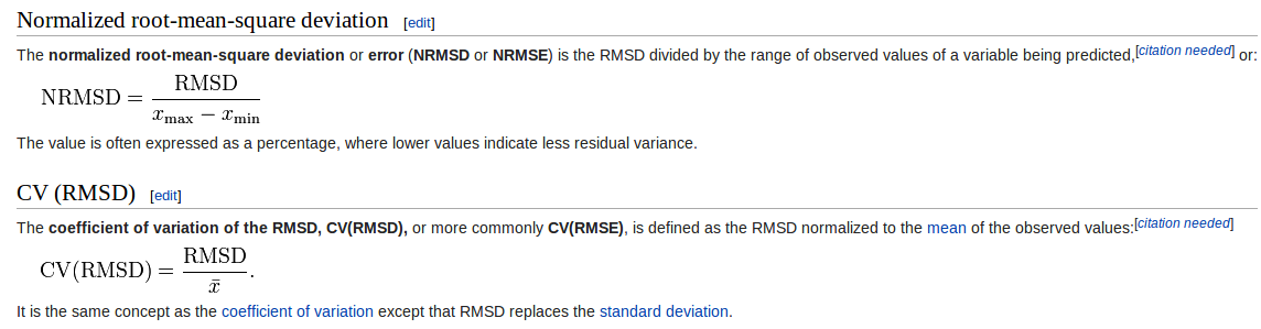
When you said in the last emails:
"normalized root-mean-square (RMS) differences"
you're talking about to normalize using the formula below:
[image: Imagem inline 1]
Thanks,
Guilherme.
2014-03-23 20:27 GMT-03:00 Dennis Shea <shea@ucar.edu>:
>
> At the top of the Taylor Diagram WWW page
> http://www.ncl.ucar.edu/Applications/taylor.shtml
>
> A link is provides to Karl Taylor's "Taylor Diagram Primer"
>
> http://www-pcmdi.llnl.gov/about/staff/Taylor/CV/Taylor_diagram_primer.pdf
>
> It is an 'easy read.' This summarizes the important aspects of these
> useful plots.
> ====
> The top of the NCL Taylor Diagram WWW page, it states:
>
> "The pertinent statistics are the weighted pattern
> correlation (pattern_cor) and the normalized
> root-mean-square (RMS) differences."
> ---
> If u have the above quantities, it is simple to plot.
> EG: Look at Example 1.
>
> --
> xc(nlat,mlon), xo(nlat,mlon)
>
> (1) You need centered pattern correlations. NCL provides
> a function for this computation:
>
>
> http://www.ncl.ucar.edu/Document/Functions/Contributed/pattern_cor.shtml
>
> (a) if the variables are on different grids, you *must* interpolate
> to a common grid. Generally, the 'common grid' is
> the control grid. Then calculate the pattern correlation.
> ---
> [2] You need the area weighted centered variances. Not necessary but
> for consistency, they should use the same grid. The following
> assumes that xo and xc are on the same grids. Taylor states:
> "... the centered root-mean-square (RMS) difference between
> the simulated and observed patterns ..."
>
> (a) Compute the weighted area means for each grid
> ; areal mean: rectilinear grid
> xavgc = wgt_areaave(xc,...,gw,..) ; control
> xavgo = wgt_areaave(xo,...,gw,..) ; 'other' dataset
> ; gw could be cos(lat)
> or
> ; areal mean: curvilinear grid
> xavgc = wgt_areaave2(xc,..,w2,..) ; control
> xavgo = wgt_areaave2(xo,..,w2,.) ; 'other' dataset
> ; w2 could be cos(lat2d)
>
> or, more explicitly, for xc and xo on the same grid: wgtc=wgto
>
> wgtc = conform_dims(dimsizes(xc), gw, 0) ; make 2d for gw[*]
>
> xavgc = sum(wgtc*xc)/sum(wgtc) ; control centered mean
> xavgo = sum(wgtc*xo)/sum(wgtc)
>
> (b) compute the sum of the centered area weighted variances.
>
> dc2 = sum(wgtc*(xc-xavgc)^2) ; control ; centered about xavgc
> do2 = sum(wgtc*(xo-xavgo)^2)
> rat = sqrt(do2/dc2)
>
>
>
> On 3/18/14, 12:58 AM, louis Vonder wrote:
> > Dear members of the NCL community,
> >
> > Here a script than I am trying to use to compare datasets.
> > It is a Taylor diagram snipped from ncl example page.
> >
> > I want know there is no mistake.
> > Particularly where I am computing pattern correlation and standard
> deviation normalization.
> >
> >
> > Regards,
> >
> >
> >
> >
> > ;**********************************
> > ; DIAGRAMME DE TAYLOR
> > ;**********************************
> > load "$NCARG_ROOT/lib/ncarg/nclscripts/csm/gsn_code.ncl"
> > load "$NCARG_ROOT/lib/ncarg/nclscripts/csm/gsn_csm.ncl"
> > load "$NCARG_ROOT/lib/ncarg/nclscripts/csm/contributed.ncl"
> > load "$NCARG_ROOT/lib/ncarg/nclscripts/csm/shea_util.ncl"
> > load "taylor_diagram.ncl"
> > ;load "taylor_metrics_table.ncl"
> > ;**********************************
> > ;**********************************
> > begin
> >
> > ;************ data reading ***************************************
> >
> >
> >
> > data0 = addfile("reg_cru_pre.nc", "r") ; CRU
> > data1 = addfile("pregpcp1998_2007_inter.daily.nc",
> "r") ;
> > data2 = addfile("
> CMAP_precip.mon.mean_inter_1998_2007.nc", "r")
> > data3 = addfile("
> precip.mon.total.v301_inter_1998_2007.nc", "r")
> > data4 = addfile("
> precip.mon.total.v6_inter_1998_2007.nc", "r")
> >
> >
> > pre0 = data0->pre
> > pre1 = data1->data
> > pre2 = data2->precip
> > pre3 = 10*data3->precip
> > pre4 = data4->precip
> >
> >
> > copy_VarAtts(data3->precip, pre3)
> >
> >
> > ;******************Pattern correlation
> ************************************
> > cor1 = dim_avg_n_Wrap(pattern_cor( pre0, pre1, 1.0, 0), 0)
> > cor2 = dim_avg_n_Wrap(pattern_cor( pre0, pre2, 1.0, 0), 0)
> > cor3 = dim_avg_n_Wrap(pattern_cor( pre0, pre3, 1.0, 0), 0)
> > cor4 = dim_avg_n_Wrap(pattern_cor( pre0, pre4, 1.0, 0), 0)
> >
> > mmd= (/cor1, cor2, cor3, cor4/)
> > print(mmd)
> > ;****************** Standard deviation **************************
> >
> > pre0_Std = dim_avg_n_Wrap( dim_stddev_n_Wrap( pre0, (/1,2/)), 0)
> > pre1_Std = dim_avg_n_Wrap( dim_stddev_n_Wrap( pre1, (/1,2/)), 0)
> > pre2_Std = dim_avg_n_Wrap( dim_stddev_n_Wrap( pre2, (/1,2/)), 0)
> > pre3_Std = dim_avg_n_Wrap( dim_stddev_n_Wrap( pre3, (/1,2/)), 0)
> > pre4_Std = dim_avg_n_Wrap( dim_stddev_n_Wrap( pre4, (/1,2/)), 0)
> >
> > print(dimsizes(dim_stddev_n_Wrap( pre4, (/1,2/))))
> >
> > ;**************** Standard deviations normalisation
> *********************
> >
> > std1 = pre1_Std/pre0_Std
> > std2 = pre2_Std/pre0_Std
> > std3 = pre3_Std/pre0_Std
> > std4 = pre4_Std/pre0_Std
> >
> > fud = (/std1, std2, std3, std4/)
> >
> > ; Cases [Model]
> > case = (/ "precipitation" /)
> > nCase = dimsizes(case )
> > ; variables compared
> > var = (/ "GPCP", "CMAP", "UDEL", "GPCC"/)
> >
> > nVar = dimsizes(var)
> >
> >
> > p_rat = (/std1, std2, std3, std4/)
> >
> > p_cc = (/cor1, cor2, cor3, cor4/)
> >
> >
> > ;**********************************
> > ; Put the ratios and pattern correlations into
> > ; arrays for plotting
> > ;**********************************
> >
> > nDataSets = 1 ; number of datasets
> > npts = dimsizes(p_rat)
> >
> > ratio = new ((/nCase, nVar/), typeof(p_rat) )
> > cc = new ((/nCase, nVar/), typeof(p_cc) )
> >
> > ratio(0,:) = p_rat
> > cc(0,:) = p_cc
> >
> >
> ;**********************************************************************************************************************
> > ;***************************** create plot
> ************************************************
> >
> ;**********************************************************************************************************************
> > res = True ;
> diagram mods desired
> > res@tiMainString = "precipitation" ; title
> > res@Colors = (/"blue"/) ; ;
> marker colors
> > res@Markers = (/14/) ;,9,2,3,8/) ;
> marker styles
> > res@markerTxYOffset = 0.03 ;
> offset btwn marker & label
> > res@gsMarkerSizeF = 0.018 ;
> marker size
> > res@txFontHeightF = 0.018 ;
> text size**************taille des lettres et chiffres******
> >
> > res@stnRad = (/ 0.75, 1.25 /) ; additional standard
> radii
> > res@ccRays = (/ 0.6, 0.9 /) ; correllation rays
> > ;res@ccRays_color = "LightGray" ; default is "black"
> >
> > res@varLabels = var
> > res@caseLabels = case ; affiche la liste des
> variables charg�es
> > res@varLabelsYloc = 1.5 ; Move location of variable
> labels [pour taylor]
> > ;res@varLabelsYloc = 1.65 ; Move location of variable
> labels [pour taylor2]
> > ;res@varLabelsYloc = 2.04 ; Move location of variable
> labels [pour taylor1]
> > res@caseLabelsFontHeightF = 0.10 ; make slight larger
> [default=0.12 ]
> > res@varLabelsFontHeightF = 0.01 ; make slight smaller
> [default=0.013]
> >
> > res@centerDiffRMS = True ; RMS 'circles'
> > res@centerDiffRMS_color = "LightGray" ; default is "black"
> >
> > wks = gsn_open_wks("eps", "pre_tailor_annual")
> > plot = taylor_diagram(wks, ratio, cc, res)
> >
> >
> ;**********************************************************************************************************************
> >
> ;**********************************************************************************************************************
> >
> ;**********************************************************************************************************************
> > end
> >
> > _______________________________________________
> > ncl-talk mailing list
> > List instructions, subscriber options, unsubscribe:
> > http://mailman.ucar.edu/mailman/listinfo/ncl-talk
> >
> _______________________________________________
> ncl-talk mailing list
> List instructions, subscriber options, unsubscribe:
> http://mailman.ucar.edu/mailman/listinfo/ncl-talk
>
--
https://sites.google.com/site/jgmsantos/
_______________________________________________
ncl-talk mailing list
List instructions, subscriber options, unsubscribe:
http://mailman.ucar.edu/mailman/listinfo/ncl-talk