NCL Home>
Application examples>
Data sets ||
Data files for some examples
Example pages containing:
tips |
resources |
functions/procedures
NCL: HDF: Hierarchical Data Format
HDF-SDS: Scientific Data Set
HDF-EOS: Earth Observing System
HDF and HDF-EOS
In 1993, NASA chose the Hierarchical Data Format Version 4 (HDF4)
to be the official format for all data products derived by the
Earth Observing System (EOS). It is commonly used for
satellite based data sets. There are several 'models' of
HDF4 which can be a bit confusing. Each model addresses
different needs. One model is the Scientific Data Set (SDS) which is
similar to netCDF-3 (Classic netCDF). It supports multi-dimensional
gridded data with meta-data including support for an unlimited dimension.
To better serve a broader spectrum within the user community
with needs for geolocated data, a new format or convention,
HDF-EOS2 was developed.
HDF-EOS supports three geospatial data types: grid,
point, and swath.
Limitations of the HDF4 format, needs for improved data compression and
changing computer paradigms led to the introduction of a
new HDF format (HDF5) in 2008. The HDF4 and HDF5 appellations
might imply some level of compatibility.
Unfortunately, no! These are completely independent formats.
The calling interfaces and underlying storage formats are different.
Unlike the netCDF community which has a well established
history of conventions
(eg., Climate and Forecast convention),
there seems to be a lack of commonly accepted conventions by the
HDF satellite community. For example the "units" for geographical coordinates under the
CF convention must be recognized by the
udunits package. Often on HDF files the latitude and longitude
variables will have the units "degrees" while netCDF's CF convention
would require "degrees_north" and "degrees_east" or some other recognized units.
Some experiments (eg,
AURA)
have developed "guidelines" for data. However, perhaps because the spectrum
of experiments is large, the HDF community does not have a "culture" where broadly accepted
conventions are commonly used.
NASA Data Processing Levels
NASA data products are processed at various
Data Processing Levels ranging from Level 0 to Level 4.
Level 0 products are raw data at full instrument resolution. At higher levels, the data
are converted into more useful parameters and formats. Often the levels are included in
the file name:
eg. L0, L1, L1A, L1B, ..., L3, L4.
NCL General Comments
NCL
recognizes and supports multiple data formats including
HDF4, HDF5, HDF-EOS2 and HDF-EOS5. The following HDF
related file extensions are recognized: "hdf", "hdfeos",
"he2", "he4", and "he5".
The first rule of 'data processing' is to look at the data.
The command line utility
ncl_filedump
can be used to examine a file's contents. Information such as a variable's type,
size, shape can allow users to develop optimal code for processing.
The stat_dispersion and
pdfx functions
can be used to examine a variable's distribution. It is not
uncommon for outliers to be present. If so, it is best to manually specify
the contour limits and spacing to maximize information content
on the plots.
A possible source of confusion is that variables that are "short" or "byte"
can be unpacked to float via two different formulations. If x
represents a variable of type "short" or "byte", the unpacked
or scaled value can be derived via:
          value =  x*scale_factor + add_offset
or
          value = (x - add_offset)*scale_factor
Examples of files that use the latter formula are at
MYDATML_2, MYD04_L2.
The NCL functions
short2flt/
byte2flt can
be used to unpack the former, while,
short2flt_hdf/
byte2flt_hdf can
be used to unpack the latter.
FYI: An Inconsistency between Reading HDF4 and HDF-EOS2
The following does not apply for NCL versions 6.2.0 and newer.
NCL v6.2.0 perform a 'double read' HDF and HDF-EOS and merges the
appropriate meta data.
An issue which may confuse users reading HDF-EOS2 files is that a variable
imported after a file has been opened with a .hdf extension may
have different meta data associated with it then if it had been imported
after being opened with a .hdfeos or .he2 extension. The reason
is that although HDF-EOS2 library has an interface for getting variable attributes,
many of the attributes that would be visible when reading using the
straight HDF library are not accessible using the HDFEOS library.
Conversely, the coordinates are often only visible using the HDF-EOS2 library. So,
currently, the only solution is for the user to examine the variable by
opening the file via each extension (ie: a 'double read').
Data used in the Examples
Regardless of the dataset used, the same principle can be used to process the data.
HDF-SDS [hdf]
   TRMM   - Tropical Rainfall Measuring Mission
   MODIS  - Moderate Resolution Imaging Spectroradiometer
   SeaWiFS- Sea-viewing Wide Field-of-view Sensor [ SeaWiFS examples ]

HDF4EOS [he2, he4, hdfeos]
   AIRS   - Atmospheric Infrared Sounder
   MODIS  - Moderate Resolution Imaging Spectroradiometer

HDF5EOS [he5]
   HIRDLS - High Resolution Dynamics Limb Sounder
   MLS    - Microwave Limb Sounder
   OMI    - Ozone Monitoring Instrument
   TES    - Tropospheric Emission Spectrometer

HDF5 [h5]
   GPM    - Global Precipitation Mission
   SMAP   - Soil Moisture Active Passive
HDF Group Comprehensive Examples
The HDF-Group has created a suite of examples called the
hdfeos.org/zoo.
It contains
NCL, Matlab, IDL and Python example scripts and the associated images.
A 'side-benefit' is that looking at these examples provides some insight on how the
different tools accomplish the same task. Caveat: Possibly, an expert in any one of these
languages could create a more elegent script and better image.
They also provide NCL specific comments.
Some HDF examples may need a library named
HDFEOS_LIB.ncl .
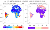
 hdf4sds_1.ncl
:
Read a TRMM
file containing 3-hourly
precipitation at 0.25 degree resolution. The geographical
extent is 40S to 40N. This data is from the
Tropical Rainfall Measuring Mission (TRMM).
Create a packed netCDF
using the pack_values function.
This creates a file half the size of those created
using float values. Some precision is lost but is not important here.
This HDF file is classifed as a "Scientific
Data Set" (HDF4-SDS).
Unfortunately, the file is not 'self-contained'.
because the file contnts do not contain the geographical coordinates
or temporal information The former must be obtained via
a web site while the time is embedded within the file name.
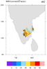
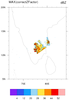
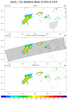
 hdf4sds_2.ncl
:
Read an
HDF4-SDS file that contains high resolution (1km)
data over India and Sri Lanka. The file does not explicitly contain
any coordinate arrays. However, the variable on the file
"Mapped_Composited_mapped" does have the following attributes:
         Slope :         1
         Intercept :     0
         Scaling :      linear
         Limit :        (    4,   62,   27,   95 )
         Projection_ID :        8
         Latitude_Center :         0
         Longitude_Center :     78.5
         Rotation :        0
The
Slope/Intercept attributes would indicate that no scaling has been
applied to the data. The
Limit attribute indicates the geographical
limits and the
Latitude_Center/Longitude_Center/Rotation
specify map attributes. The variable does not specify any
missing value [_FillValue] attribute but, after looking at the
data, it was noted that the value -1 is appropriate.
The stat_dispersion function was
used to determine the standard and robust estimates of the
variable's dispersion. Outliers are present and the contour
information was manually specified.
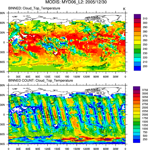
 hdf4sds_3.ncl
: Read multiple files
(here, 131 files) for one particular day; for each file
bin and sum the satellite data using
bin_sum;
after all files have been read, use
bin_avg
to average all the summed values; plot; create a netCDF
of the binned (gridded data).
Note:
Here the data are netCDF files. However, the original files were
HDF-SDS (eg: MYD06_L2.A2005364.1405.005.2006127140531.hdf). The
originating scientist converted these to netCDF for some reason.
NCL can handle either. Only the file extension need be changed
(.nc to .hdf).
 hdf4sds_4.ncl
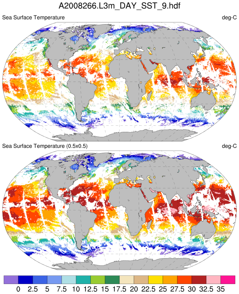
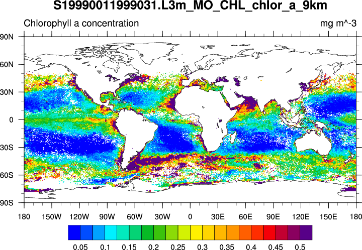
:
Read a HDF-SDS dataset containing
MODIS Aqua Level-3 SSTs. The file attributes contain the
geographical information and this is used to generate
coordinate variables. One issue is that the data "l3m_data"
are of type "unsigned short". These are not explicitly supported
through v5.1.1 (but will be in 5.2.0). Hence, a simple 'work-around'
is used.
In addition to plotting the original 9KM data, the
area_hi2lores is used to interpolate
the data to a 0.5x0.5 grid. A netCDF file is created.
Other 'L3' datasets could be directly used in the sample script.
For example: Example 3 on the
SeaWiFS Application page.
 hdf4sds_5.ncl
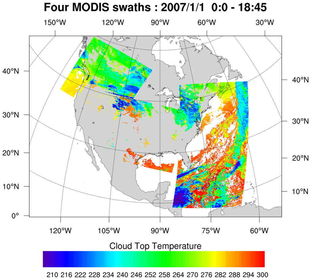
:
Read four MODIS HDF datasets and create a series
of swath contours over an Orthographic map. The 2D lat/lon data
is read off of each file and used to determine where on the map
to overlay the contours.
This example uses gsn_csm_contour_map to create the map plot
with the first set of contours, and then creates the remaining contour
plots with gsn_csm_contour. The
overlay procedure is then used to overlay these
remaining contour plots over the existing contour/map plot.

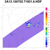
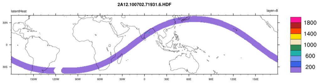
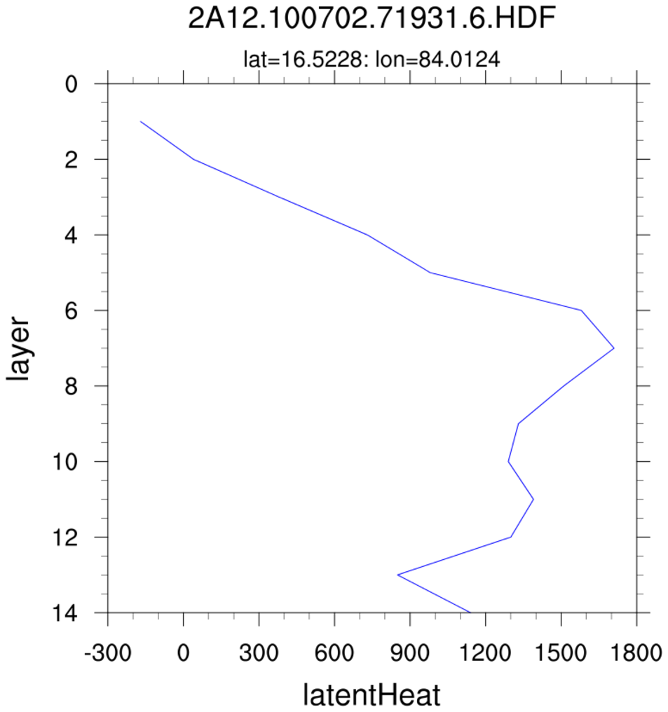
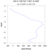 hdf4sds_6.ncl
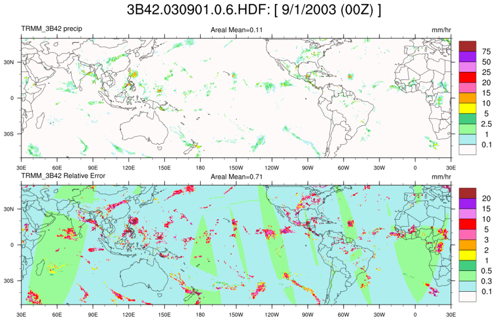
:
TRMM 2A12:
TMI Hydrometeor (cloud liquid water, prec. water, cloud ice, prec. ice) contains profiles in 14 layers at 5 km horizontal resolution, along with latent heat and surface rain, over a 760 km swath.
Specify a variable (here, "latentHeat") and plot (a) the entire swath; (b) region near India; (c) a vertical profile at locations where the latent heat
exceeds 1500. The file contains no units information for the variables.
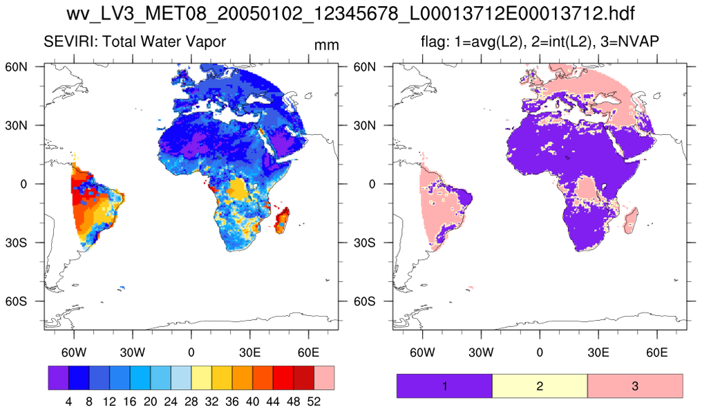
 hdf4sds_7.ncl
:
A SEVIRI Level-3 water vapor data set. The variable is packed in a rather unusual
fashion. The flags should be viewed to determine the source of the data.

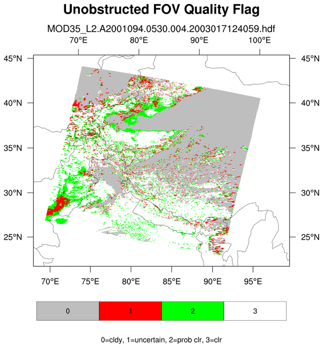
 hdf4sds_8.ncl
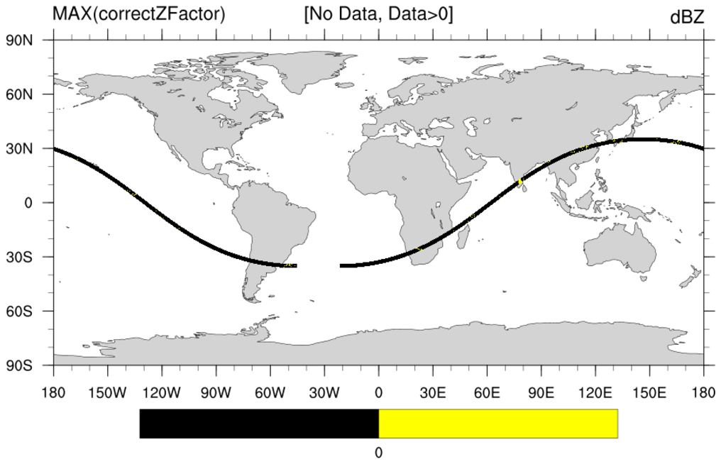
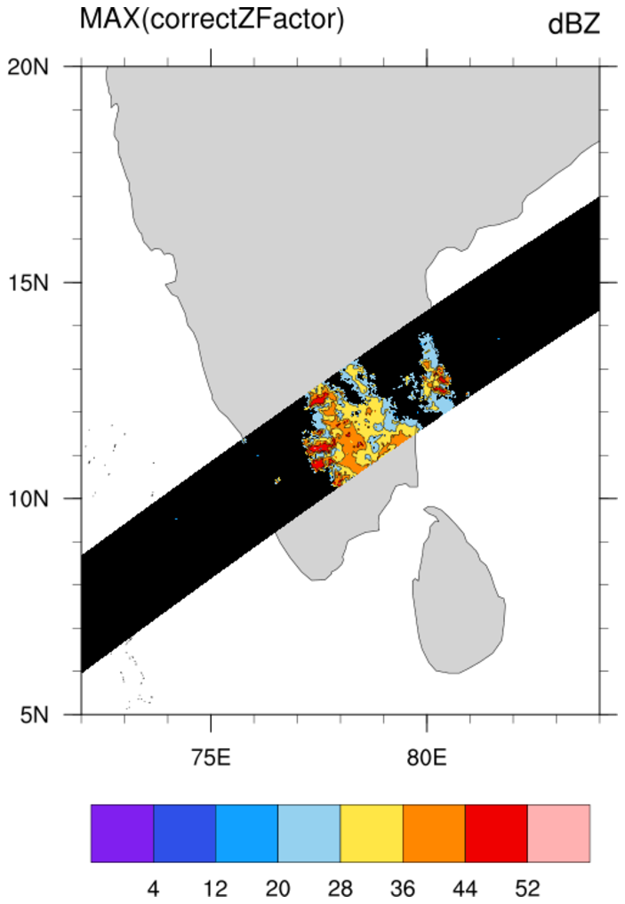
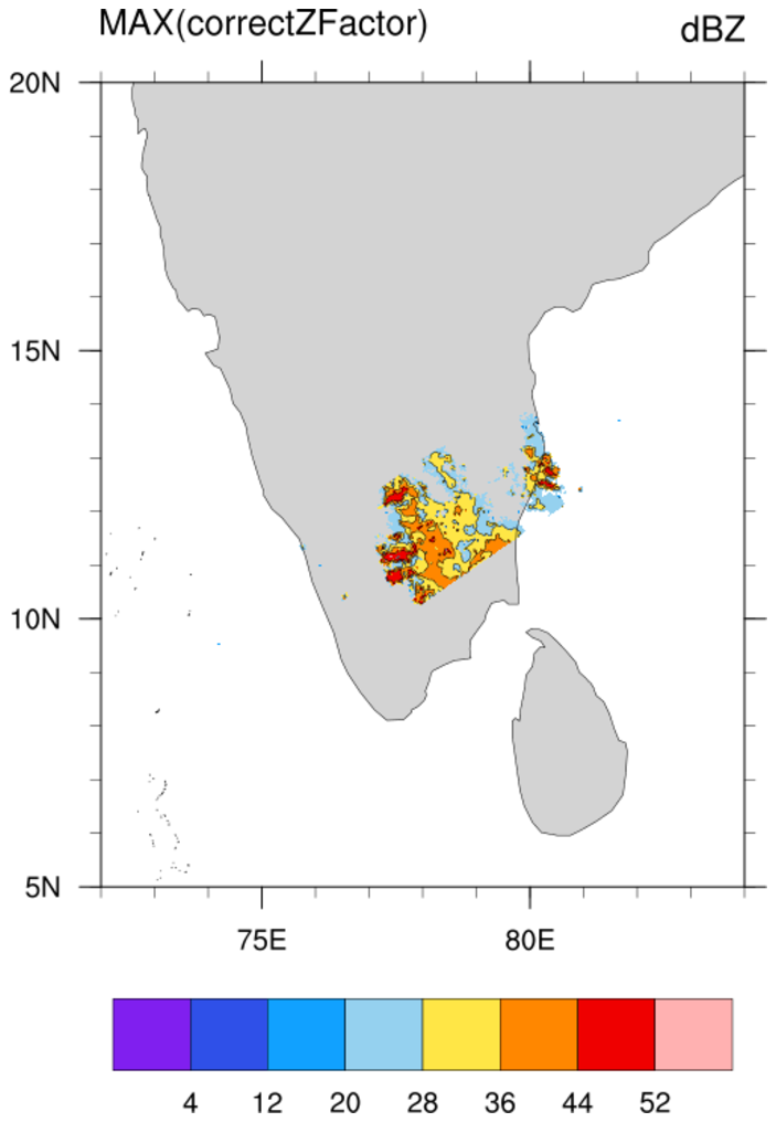
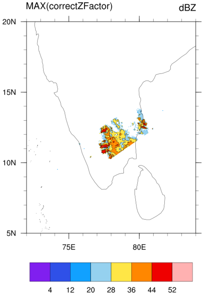
:
A TRMM A25 file is read. At each pixel, the maximum 'correctZFactor' from all levels is extracted using
dim_max_n. Several ways of presenting the data for a swath are illustrated.
 hdf4sds_9.ncl
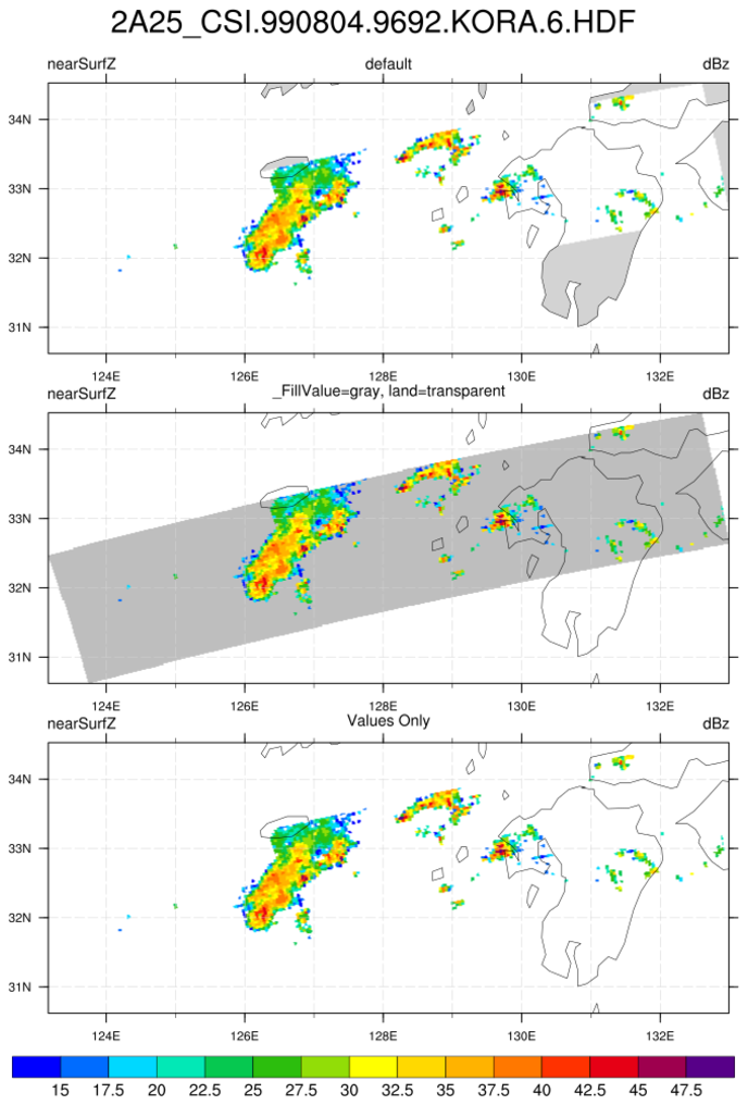
:
A TRMM A25 file is read. The 'nearSurfZ' is imported. Several ways of presenting the data for a swath are illustrated.
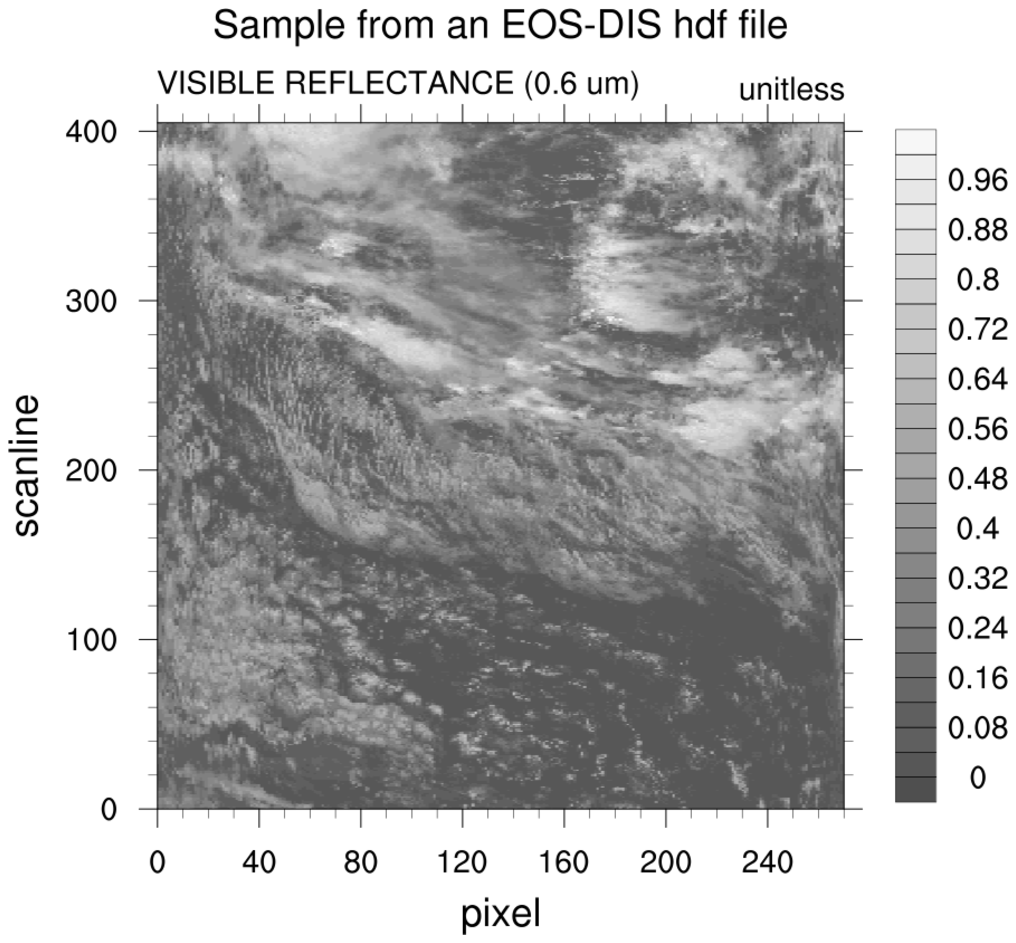
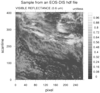 hdf4eos_1.ncl
:
Read a
HDF-EOS2 file containing
swath data.
NCL identifies the swath as
MODIS_SWATH_Type_L1B.
Create a simple plot of reflectance with coordinates of scanline
and pixel.
The eos.hdf that appears as the file name is an alias for
MOOD021KM.A2000303.1920.002.2000317044659.hdf. It is not
uncommon for a HDF-EOS2 file to have the ".hdf" file extension.
In this case, NCL will open and read the file sucessfully but
it is best to manually append the ".hdfeos" extension when opening
the file in the addfile function.
ncl_filedump eos.hdf
yields
     filename:       eos
path:   eos.hdf
   file global attributes:
      HDFEOSVersion : HDFEOS_V2.6
      StructMetadata_0 : GROUP=SwathStructure
        GROUP=SWATH_1
                SwathName="MODIS_SWATH_Type_L1B"
                [...SNIP...]
        END_GROUP=SWATH_1
END_GROUP=SwathStructure
[...SNIP...]
 hdf4eos_2.ncl
:
Example of a radiance plot. Note that the color table is reversed
from example 1.
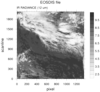
 hdf4eos_3.ncl
:
A multiple contour plot of other quantities on the MODIS file.
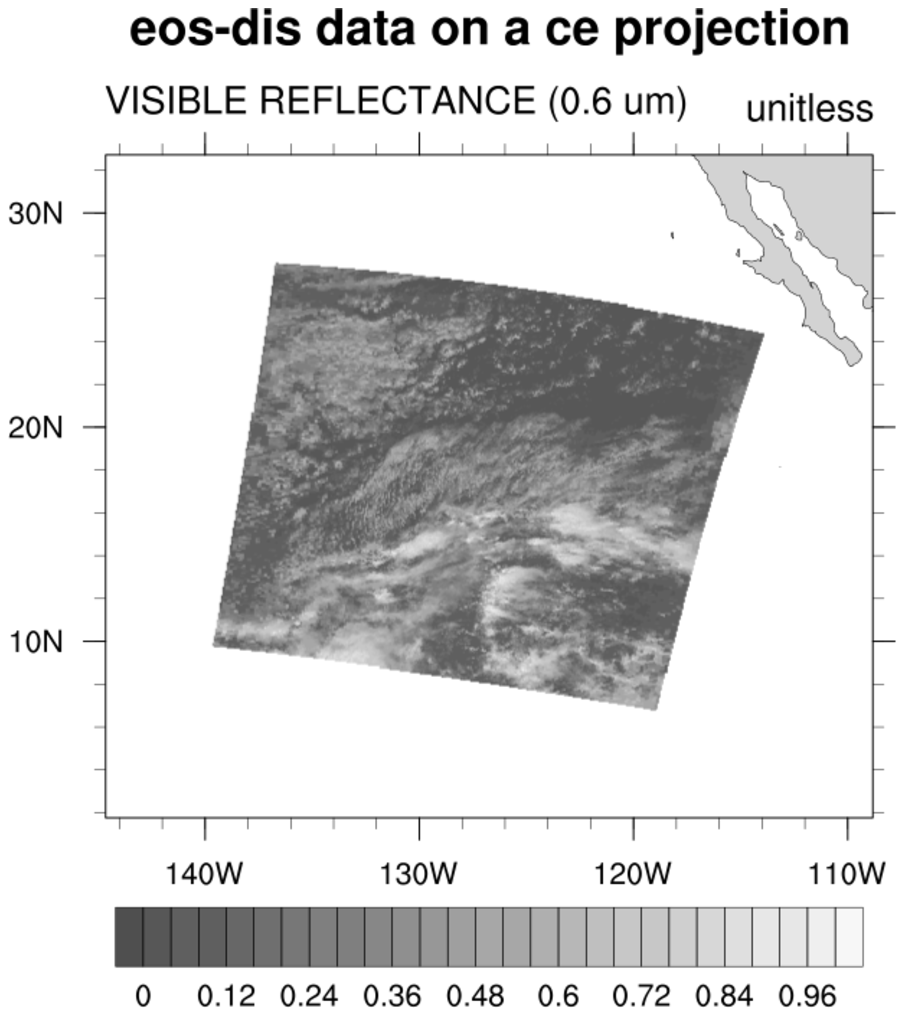
 hdf4eos_4.ncl
:
MODIS data placed on a geographical projection.
A rather awkward aspect of this file is that the Latitude and Longitude
variables differ in size from the variable being plotted.
The 5 added to the map limits is arbitrary (not required). Here it is
used to specify
extra space around the plot.
 hdf4eos_5.ncl
:
Illustrates the use of
dim_gbits to extract specic bits within a bit-stream.
A data (variable) issue is that the cloud mask variable is on a 1-km grid while the latitude/longitude
variables are on a 5-km grid. NCL array syntax (::5) is used to decimate (sub-sample) the 1-km array to the 5-km array)
It also demonstrates explicitly labeling different label bar colors with a specific integers.
The use of res@trGridType =
"TriangularMesh" makes the plotting faster.
NCL 6.5.0 introduces a new function, get_bitfield,
that will simplify the use of
dim_gbits. hdf4eos_5a.ncl
illustrates the use of this new function to obtain the same result.
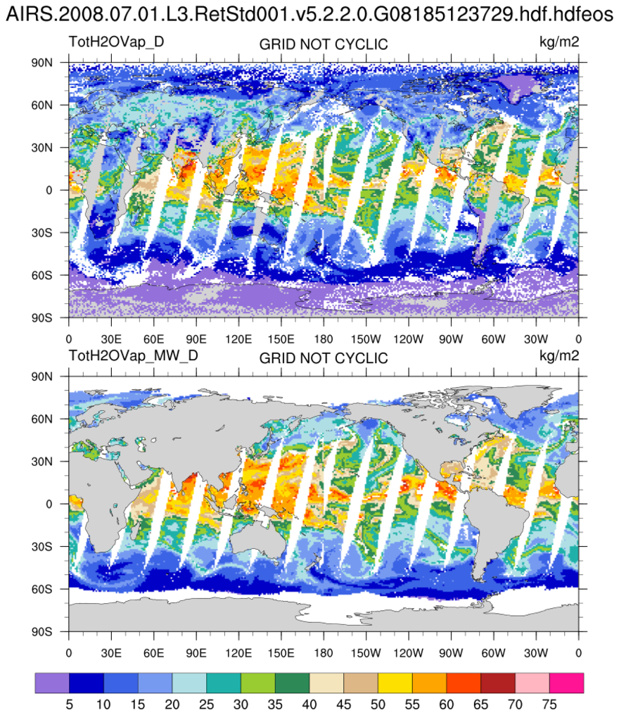
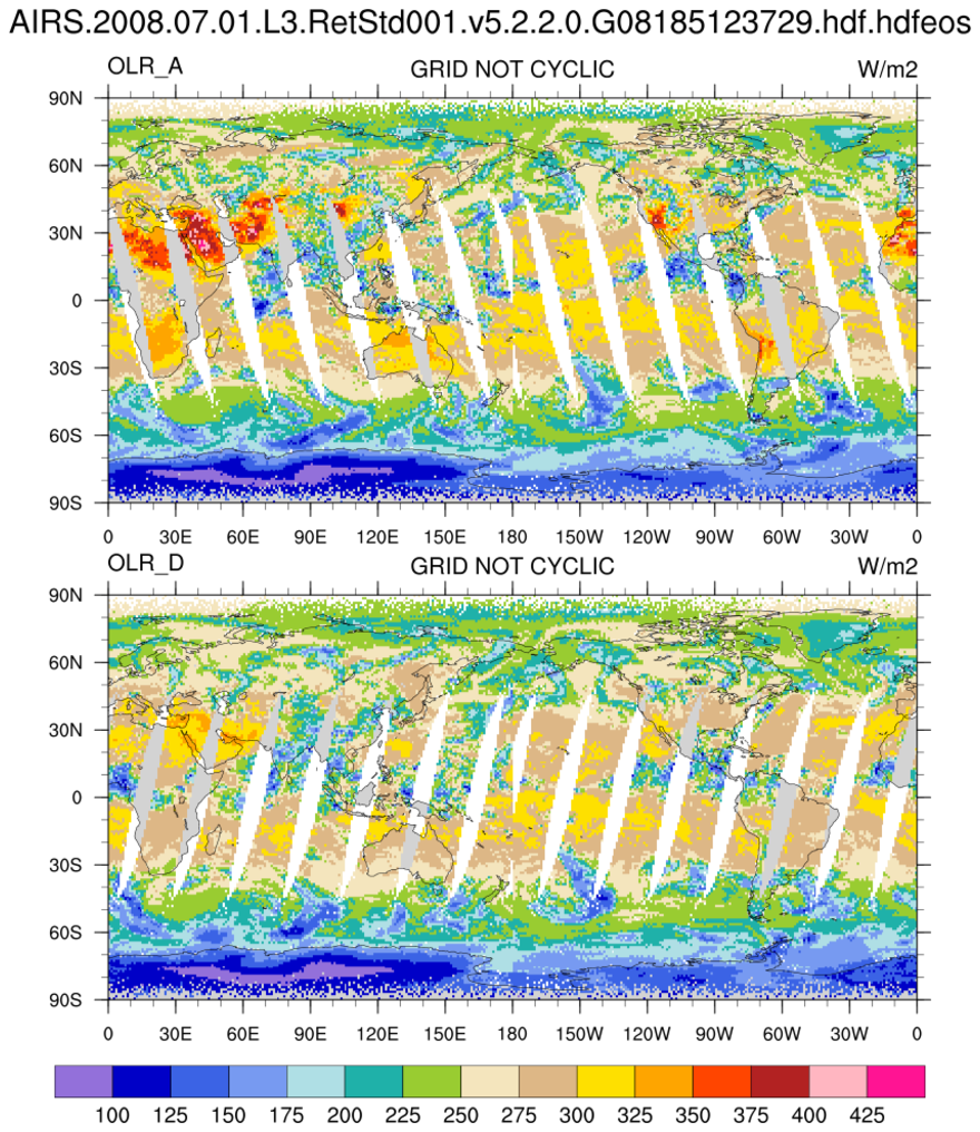
 hdf4eos_6.ncl
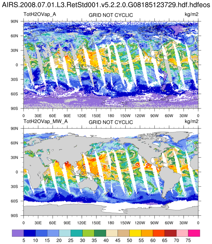
:
Read an AIRS Level-3 file (here, product type AIRX3STD). This uses the
AIR IR and MSU instruments. Although on a 1x1 degree grid, the
grid point values represent satellite swaths that have been
binned over a period of time (24 hours). The data to the left and right
of the Date Line represent
values that were sampled at different times. Hence,
the gridded
values are not cyclic in longitude.
Support for HDF5 and HDF-EOS5 is present in
v5.2.0 which was released April 14, 2010. Some samples follow.
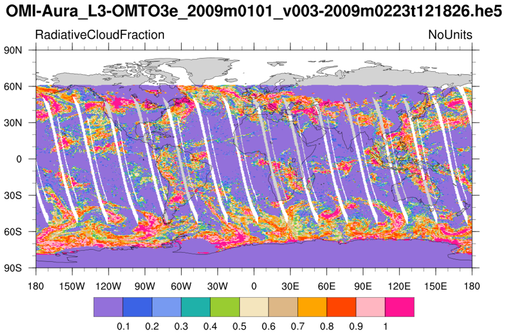
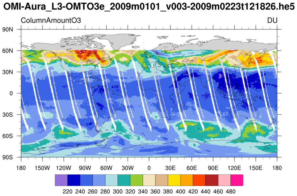
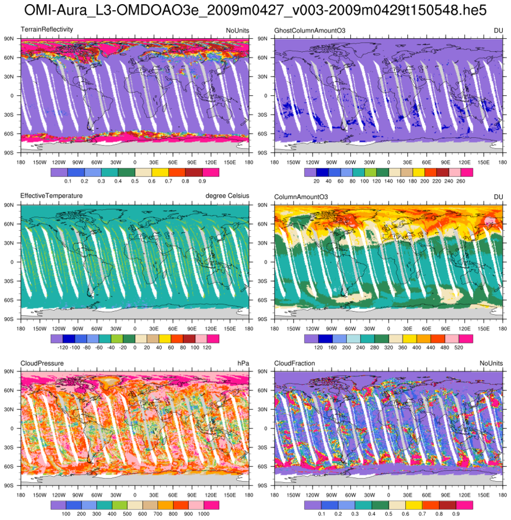
 hdf5eos_1.ncl
:
Read a
HDF-EOS5 (available v5.2.0) file from the Aura
OMI (Ozone Monitoring Instrument) and plot all the variables
on the file. Here only two of the variables are shown.
 hdf5eos_2.ncl
:
Read an
HDF-EOS5 (available v5.2.0)
file (OMI) and plot selected variables
on the file. (The
ncl_filedump
utility was used to preview the file's contents,)
This example also demonstrates how to retrieve a
variable's type prior to reading it into memory. (See
getfilevartypes.)
It is best to use
short2flt or
byte2flt if
the variable type is "short" or "byte".
These functions will automatically apply the proper scaling.
Note that the units for the "EffectiveTemperature"
variable appear to be incorrect. They indicate "degrees Celsius"
but the range would indicate "degrees Kelvin". This could be addressed
by adding the following to the script after the variable has
been imported:
     if (vNam(nv).eq."EffectiveTemperature_ColumnAmountO3") then
         x@units = "degrees Kelvin"       ; fix bad units
     end if
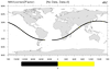
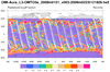
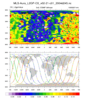
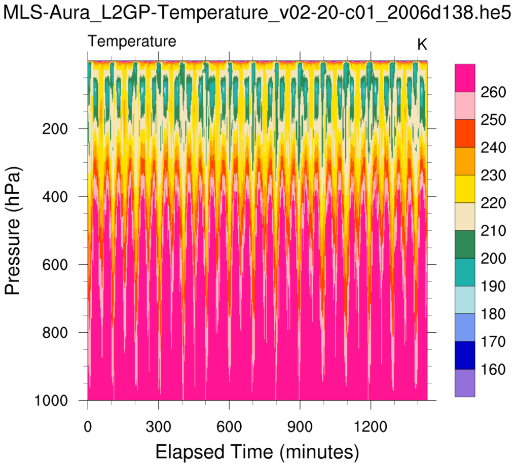
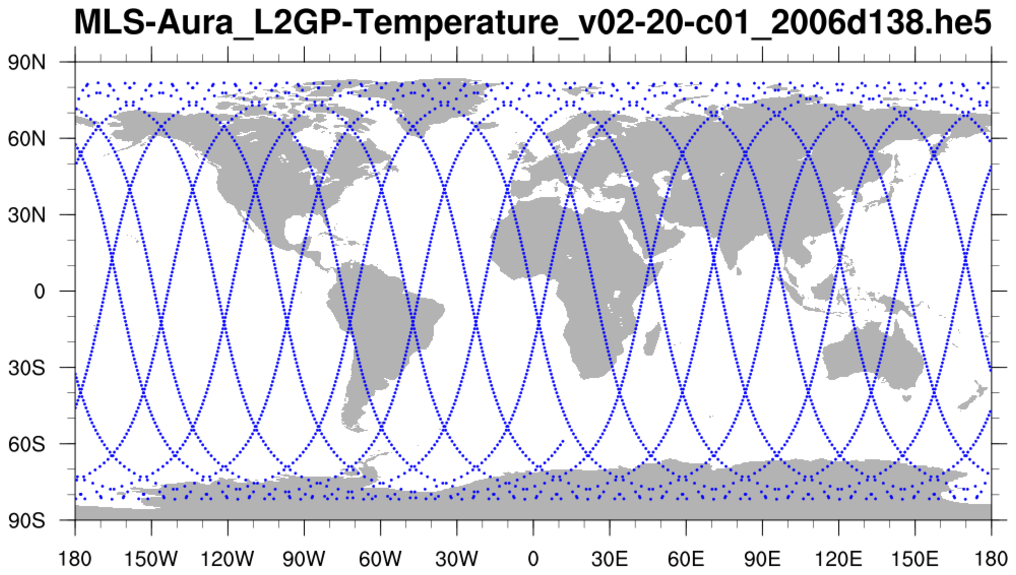
 hdf5eos_3.ncl
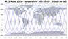
:
Read an
HDF-EOS5 (available v5.2.0) file from the MLS (Aura Microwave Limb Sounder) and
plot a two-dimensional cross-section (pressure/time) of temperature. Then plot the trajectory of the satellite over this time.
Sean Davis (NOAA) has put together a gridded satellite WV/ozone product called
SWOOSH that includes MLS data.
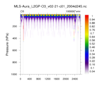
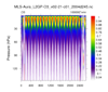
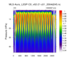
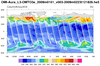
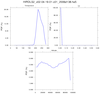
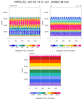
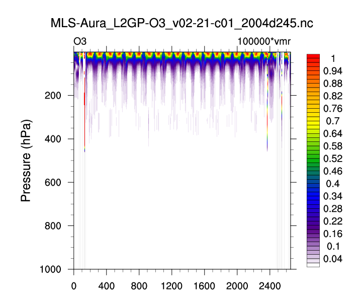
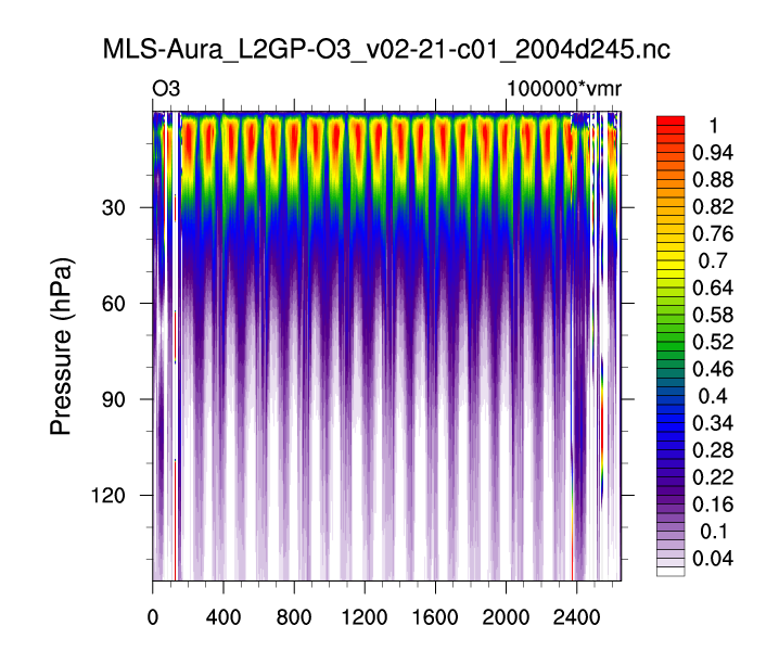
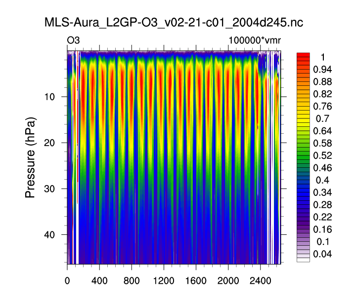
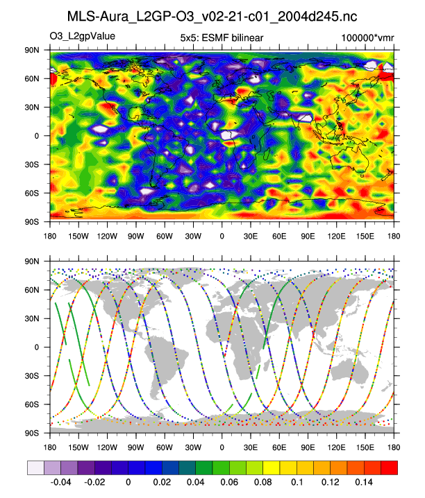
 hdf5eos_3a.ncl
:
Very similar to the previous example: (a) Different data set (MLS-Aura_L2GP-O3); (b) trajectory values are colored by value. The 3 left figures show the vertical profile of O3 along the trajectory for (i)
all levels; (b) a smaller subset; and (c) a very small subset. A user requested an example of gridding the sparsely sampled trajectory data. Obviously it was not a 'nice' picture.
Sean Davis (NOAA) has put together a gridded satellite WV/ozone product called
SWOOSH that includes MLS data.
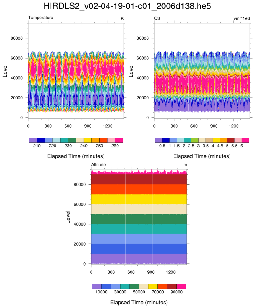
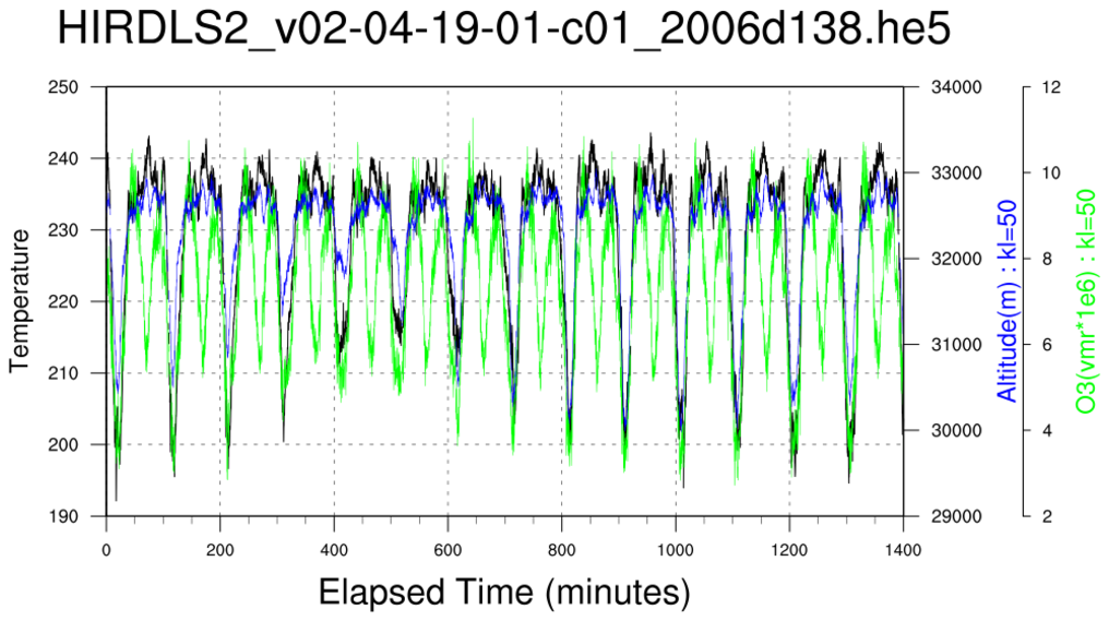
 hdf5eos_4.ncl
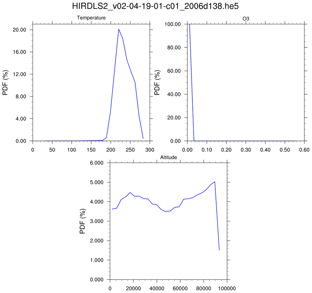
:
Read an
HDF-EOS5 (available v5.2.0) file from
the HIRDLS: (a) Use
stat_dispersion to
print the statistical information for each variable; (b) compute PDFs
via
pdfx;
(c) plot cross-sections; and, (d) plot time series of three different variables.
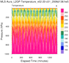
 hdf5eos_5.ncl
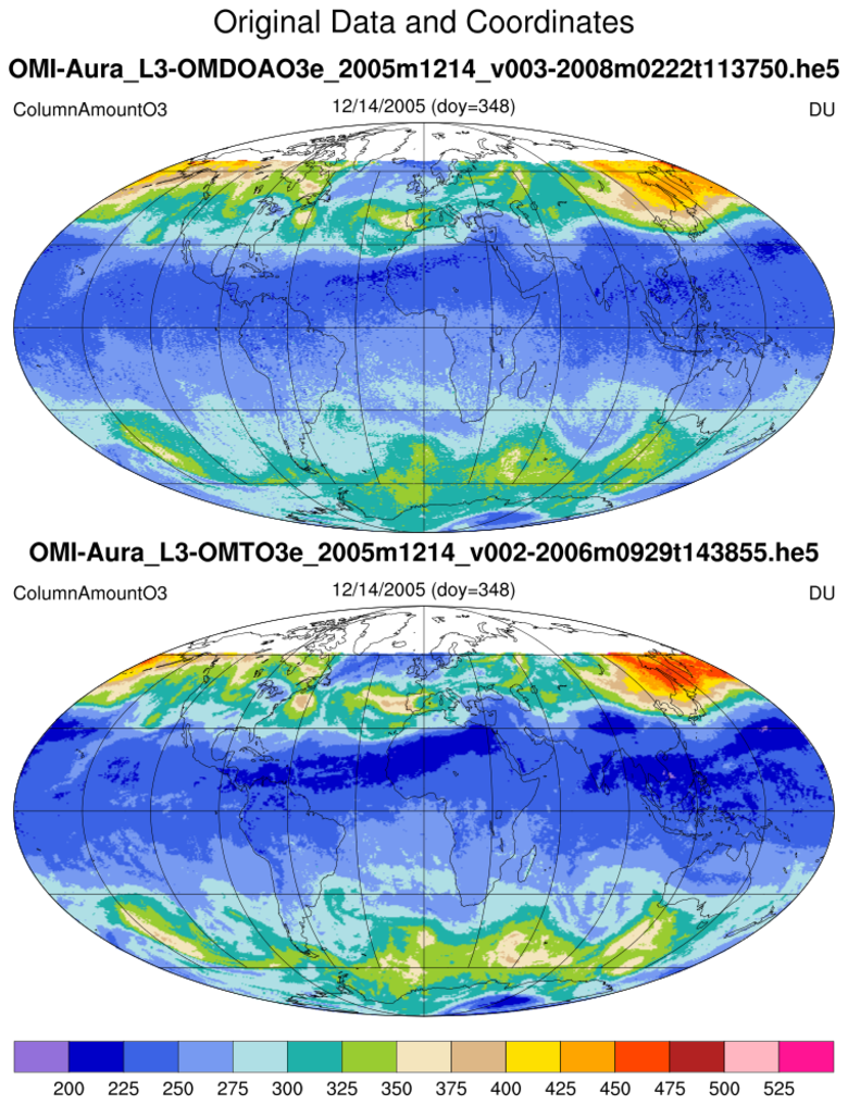
:
Read two similar OMI files (L3-OMDOAO3e and L3-OMTO3e).
This illustrates that users
must
look at a file's contents before using. (Use
ncl_filedump)
Here, there are two
files with similar variables but NCL assigns slightly different names.
The OMI L3 files used in this example have a bug in the way the OMI
data were written to the
files. NCL version 6.1.0 and
later will be able to identify OMI data files and will automatically
correct for the latitude reversal.
 amsr_1.ncl
:
Swaths containing soil moisture from the Advanced Microwave Scanning Radiometer (AMSR)
are read from multiple
h5 files. Documentation was not available but there were file 'issues':
(1) The variable name has a space ("Geophysical Data"); (2) The variable has an attribute
FillValue and not
_FillValue;
(3) There are two 'missing value categories' (-32767
s, -32768
s)
(4) The unrecognized unpacking attribute ["SCALE FACTOR"] to must be
converted to "scale_factor" for use by NCL's
short2flt function.
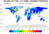
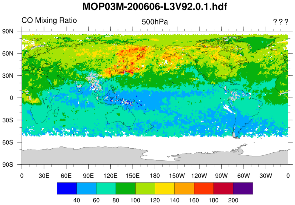
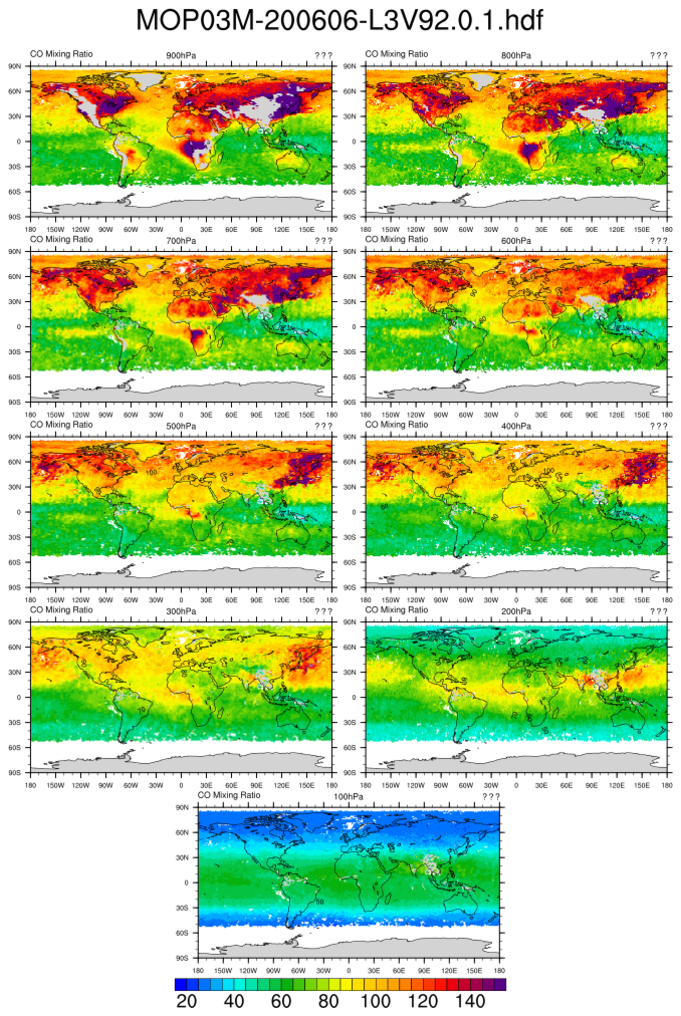
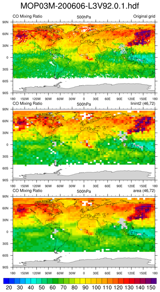
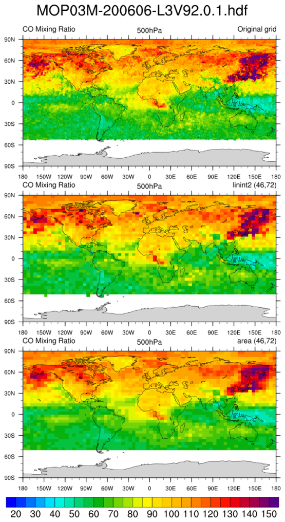
 MOPITT_MOP03M_1.ncl
:
Read a variable and plot a user specified level. The grid is (180x360).
Missing values are present. A common issue with
HDF files is that they do not contain all the desired information
or units. Hence, they must be manually provided.
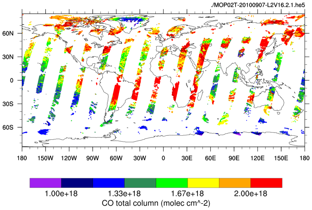
 MOPITT_MOP02T_1.ncl
:
Reads "CO Total Column" across a time interval and a selected spatial
region, and plots it on a map using a range of colored markers.
This script was contributed by Rebecca Buchholz, a researcher in the
Atmospheric Chemistry Division at NCAR.
 hdf5_1.ncl
:
Read a variable and plot it according to a palette specified on the file.
The MSG (Meteosat Second Generation) file is HDF5.
The desired variables contain a dash and a space
which are not allowed in NCL variable names. Hence,
the variables are enclosed in quotes to make them
type string. For the
-> file syntax operator
to successfully access the string variables, they must be enclosed
within dollar sign (
$).
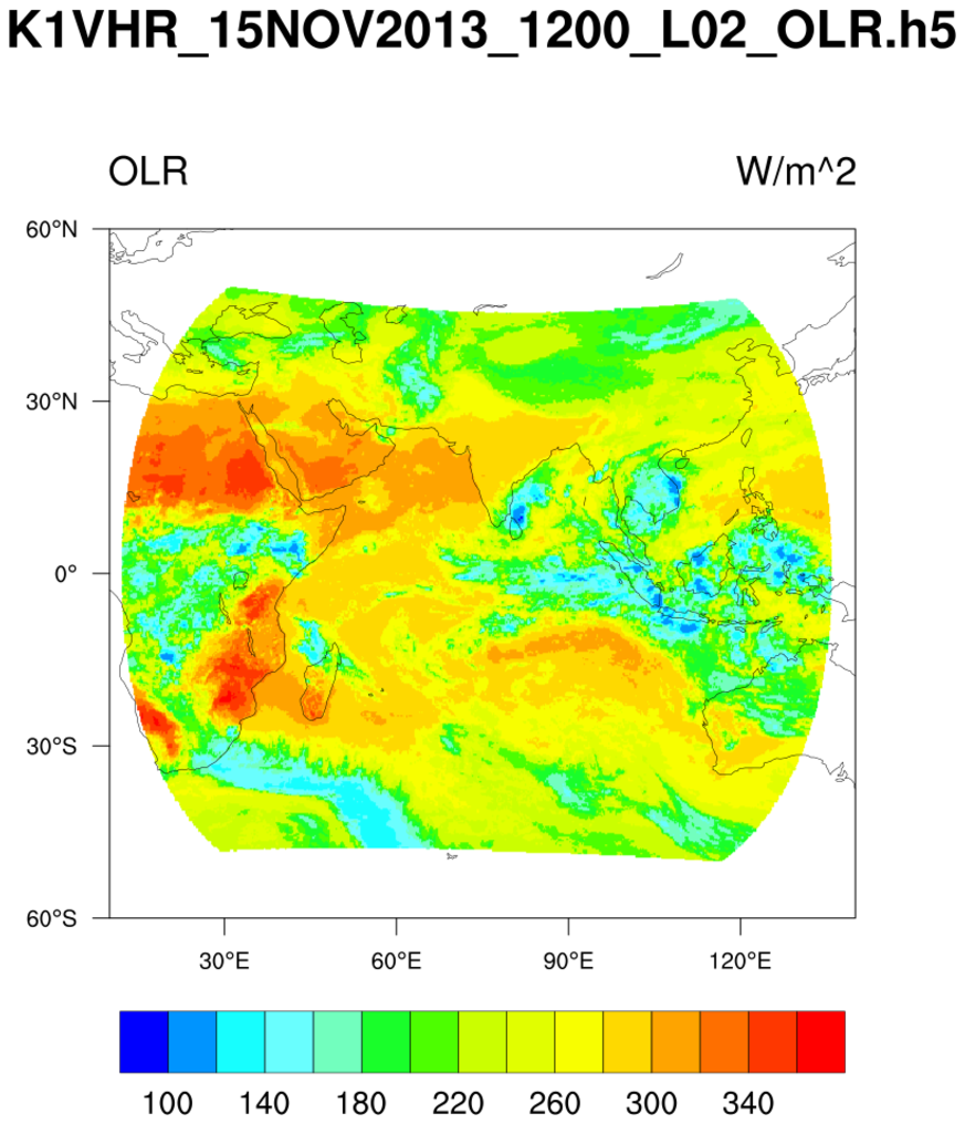
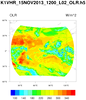 hdf5_2.ncl
:
HDF5 (h5) files can be complicated. Users should become acquainted
with the file's contents prior to creating a script.
An
ncl_filedump of the file would yield:
   %> ncl_filedump K1VHR_15NOV2013_1200_L02_OLR.h5 | less

      Variable: f
      Type: file
      filename:       K1VHR_15NOV2013_1200_L02_OLR
      path:   K1VHR_15NOV2013_1200_L02_OLR.h5
         file global attributes:
         dimensions:
            DIM_000 = 250601

         variables:
            group </OLR>

            compound <OLR_Dataset>    (Latitude, Longitude, OLR) (DIM_000)

            group </OLR/GP_PARAM_INFO>

               GP_PARAM_DESCRIPTION : Every_Acquisition
               GP_PARAM_NAME :        Outgoing Longwave Radiation (OLR)
               Input_Channels :       TIR
               LatInterval :  0.25
               Latitude_Unit :        Degrees
               LonInterval :  0.25
               Longitude_Unit :       Degrees
               MissingValueInProduct :         999
               OLR_Unit :     Watts/sq. met.
               ValidBottomLat :        -60
               ValidLeftLon :   10
               ValidRightLon :         140
               ValidTopLat :    60

            group </PRODUCT_INFORMATION>

               GROUND_STATION :       BES,SAC/ISRO,Ahmedabad,INDIA.
               HDF_PRODUCT_FILE_NAME :        K1VHR_15NOV2013_1200_L02_OLR.h5
               OUTPUT_FORMAT :        hdf5-1.6.6
               PRODUCT_CREATION_TIME :        2013-11-15T18:01:49 _L02_OLR.h5
               STATION_ID :   BES3-11-15T18:01:49 _L02_OLR.h5
               UNIQUE_ID :    K1VHR_15NOV2013_1200_L02_OLR.h5

            group </PRODUCT_METADATA>

            group </PRODUCT_METADATA/PRODUCT_DETAILS>

               ACQUISITION_DATE :     15NOV2013
               ACQUISITION_TIME_IN_GMT :      1200V2013
               PROCESSING_LEVEL :     L020V2013
               PROCESSING_SOFTWARE :  InPGS_XXXXXXXXXXXXXX
               PRODUCT_NAME : GP_OLR         XXXXX
               PRODUCT_TYPE : GEOPHY
               SENSOR_ID :    VHRPHY
               SPACECRAFT_ID :        KALPANA-1
Read a h5 (HDF5) file with 'group' fields. Note the syntax used by NCL.
The Latitude, Longitude and OLR are one-dimensional arrays of size 250601.
There are no general file conventions for HDF5 files. Users must
examine the file's contents and explicitly extract desired information.
The region of the globe is defined as attributes of the
group /OLR/GP_PARAM_INFO. These are used to create rectilinear
grid coordinates which are associated with the variable to
be plotted (olr) and written to a netCDF file.
FYI: It is not necessay to make a two-dimensional grid.
NCL can plot one-dimensional latitude/longitudinal/values
with appropriate graphical resource settings. However,
since a script option is to create a netCDF file. It
was designed to create the variable as a conventional
two-dimensional array.
 seawif_4.ncl
:
Read a SeaWIFS variable and use meta data contained within the file attributes
to construct a complete (ie, self contained) variable. The initial look at the
file was via the
ncl_filedump command line operator.
Data files were obtained
here.
Additional SeaWIFS examples are available here.
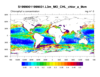
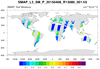
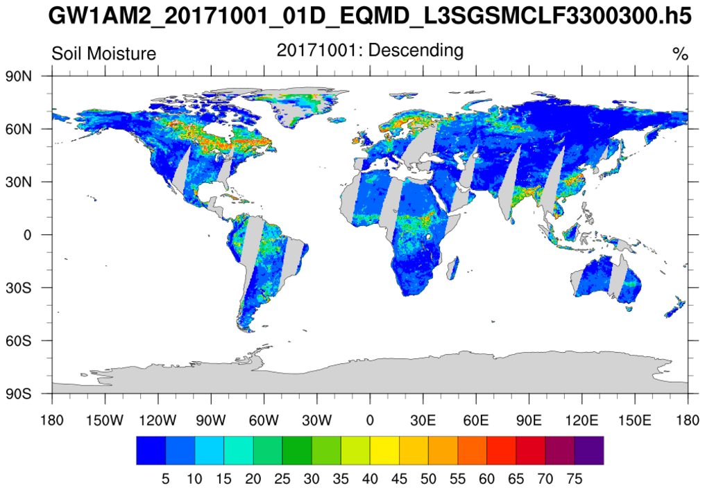
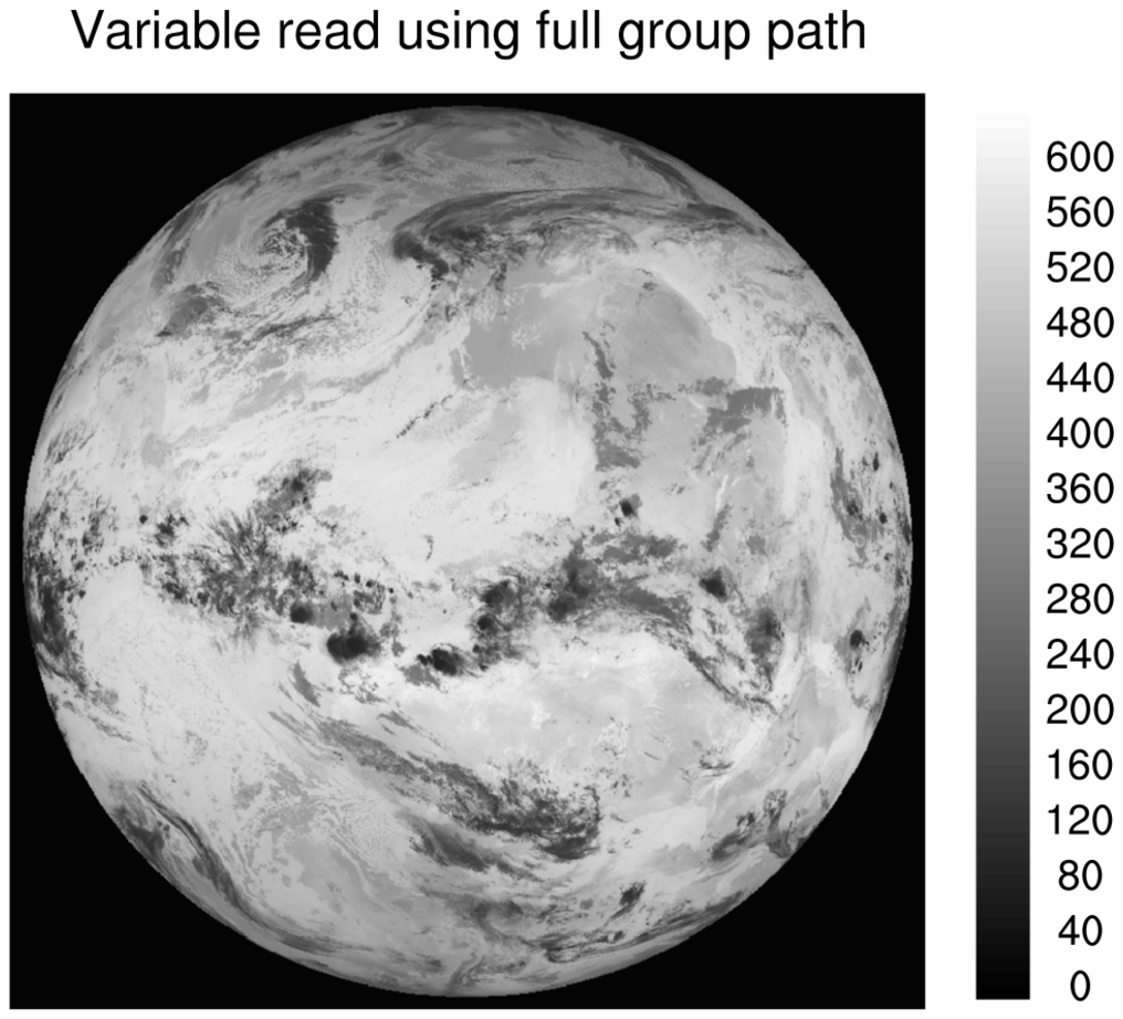
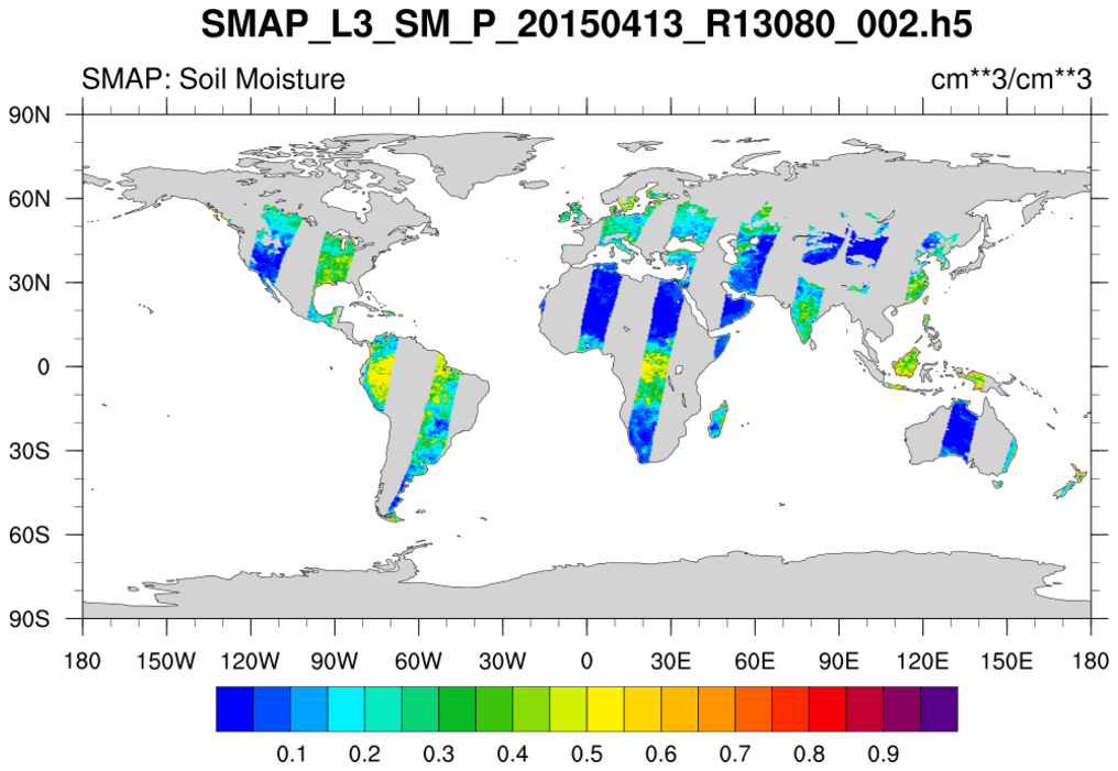
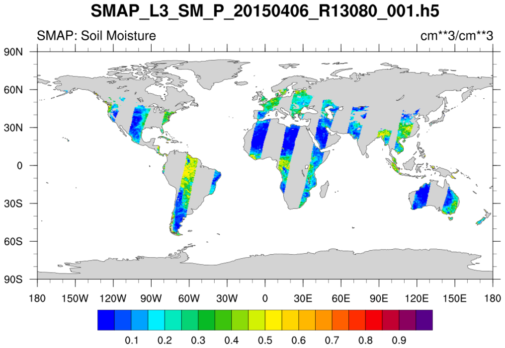
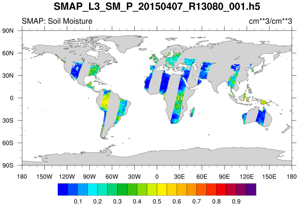
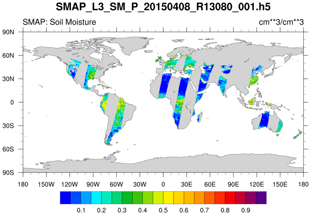
 smap_l3_1.ncl
:
NOTE:
It is recommended that users use
ncl_filedump to carefully examine
the SMAP level-3 (l3) file prior to use. Note the 'complexity' of the file. Assorted variables are
within 'groups.' NCL offers two ways to access data within groups. This and other examples
use the 'full path' method. (see script)
Read soil moisture from an individual H5 SMAP level-3 (l3) file. The data are on a regular grid BUT
the data is from a swath. The desired variable is named 'soil_moisture'.
It is located within the group named Soil_Moisture_Retrieval_Data.
The latitude and longitude variables are within this group also. A peculiarity is that the 'latitude'
and 'longitude' variables do not have an _FillValue attribute associated with them. However, a
printMinMax indicates a minimum value of -9999.0 for each. The script
assigns these manually.
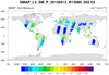
 smap_l3_2.ncl
: Similar to
smap_l3_1. The difference
is that this read mutiple files. The files are processed one-by-one. Only the first three of
of nine SMAP files are shown.
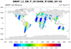
 smap_l3_3.ncl
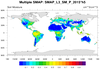
: This loops over the nine files for a particular period and
creates a composite plot by overlaying individual graphical swath grids.
Setting,
res@cnMissingValFillColor= "Transparent", keeps plotting from previous grids
from being overwritten.
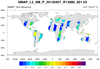
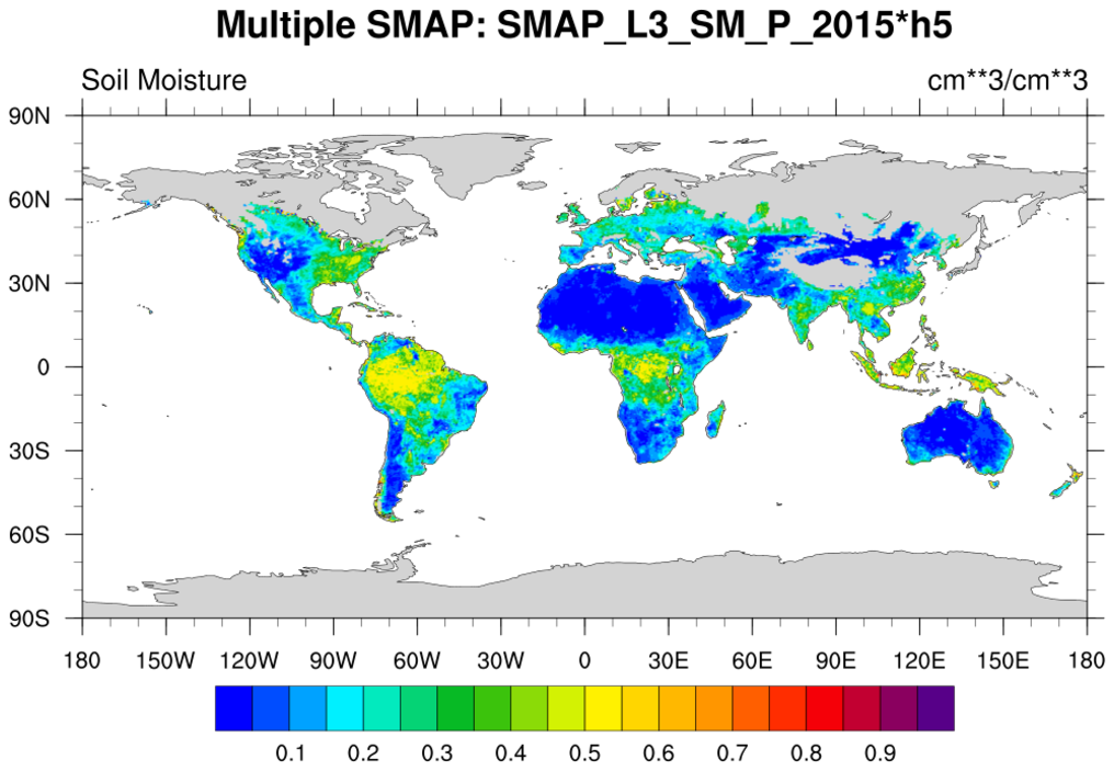
 smap_l3_4.ncl
: Similar result to
smap_l3_3.ncl.
However, it is obtained via a different method. A 'super variable' is create and the grid points are filled by use of a
where function. After reading the EASE latitude and longitude variables from
a separate file (SMAP_EASE.406x964.nc), the resulting super variable is plotted.


