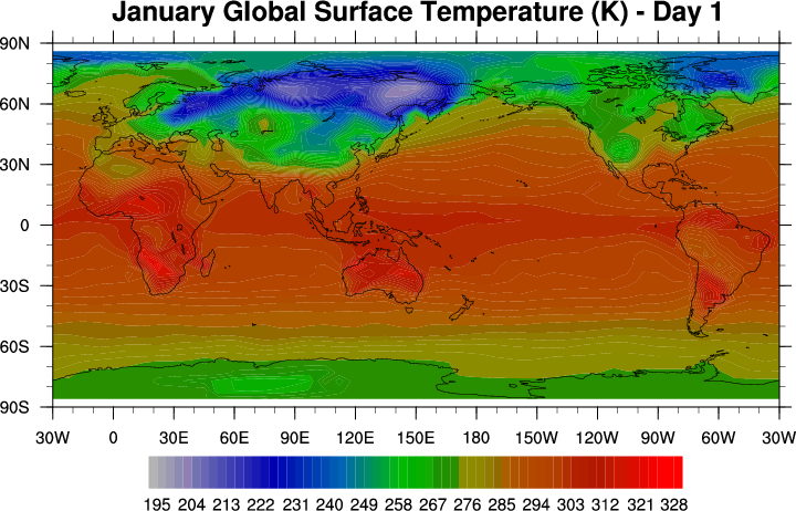
NCL Graphics: Animations

This page shows how to create animations with NCL.

If you just want to view the animation quickly and don't need to share it with somebody else, then you can send the graphical output to an NCGM file (using "ncgm" as the first argument to gsn_open_wks), and then use idt to animate it.

If you want to share the animation with other people, then you can convert from a series of NCL PNG/EPS files (or a single PS file) to an animated GIF or MPEG file using the popular "convert" tool from ImageMagick, a graphical suite for image manipulation.

For example, to convert a series of PNG images to an animated GIF with a delay of half a second between frames (50/100):

   convert -delay 50 *.png anim.gif

You can then display "anim.gif" in your browser or other suitable viewer.

For more information, see:

http://www.imagemagick.org/Usage/anim_basics/

To convert to an mpeg file, you will need to first download the program "mpeg2encode" from http://www.mpeg.org/, and then you can use "convert" again:

   convert file.ps file.mpg

animate_1.ncl: Demonstrates how to efficiently create an animation with NCL. Instead of calling gsn_csm_contour_map every time inside the "do" loop, you can use a setvalues call to just change the data and the title.

This example creates a file called "animate.ncgm". You can use idt to animate it.

   idt animate.ncgm

Three panels should pop up, and one of them has an "animate" button. Click on this, and each frame will be loaded into memory. When this is done, click the ">>" or "<<" button to play the animation. Use "delay" to slow down the animation, or "loop" to repeat it.

[View the animation.]

animate_2.ncl: Demonstrates how to create an animated GIF from WRF data.

Note that it's important set the contours to a fixed set of levels, otherwise the contour levels will be recalculated for each frame, based on the range of the data for that frame.

The output is sent to a series of PNG files, and then the following command is executed in the NCL script to produce the animation:

  convert -delay 25 animate*.png animate_2.gif

[View the animation.]

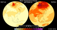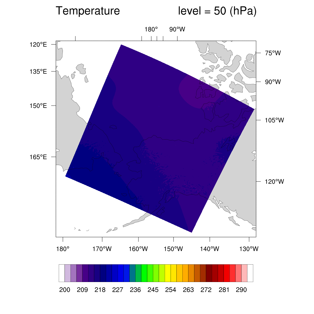
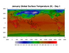
The NCL script: This animation script was contributed by Karin Meier-Fleischer of Deutsche Klimarechenzentrum (DKRZ). It shows a mean temperature change animation of CMIP5 data. It is similar to an Avizo animation, also created by DKRZ.

The images were generated as a series of PNG files, which were then converted to a ".mov" file using Adobe Photoshop Premiere. Further details on how the animation was created are included in the comments at the top of the script.

Click on the image to view the animation.

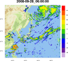
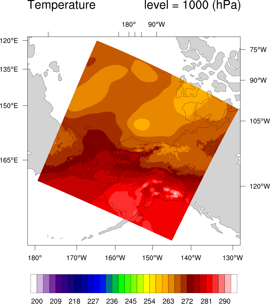
animate_3_1.ncl /
animate_3_2.ncl /
animate_3_3.ncl:

This example shows three ways to create a 97-frame animation in NCL, with tips on how to speed things up.

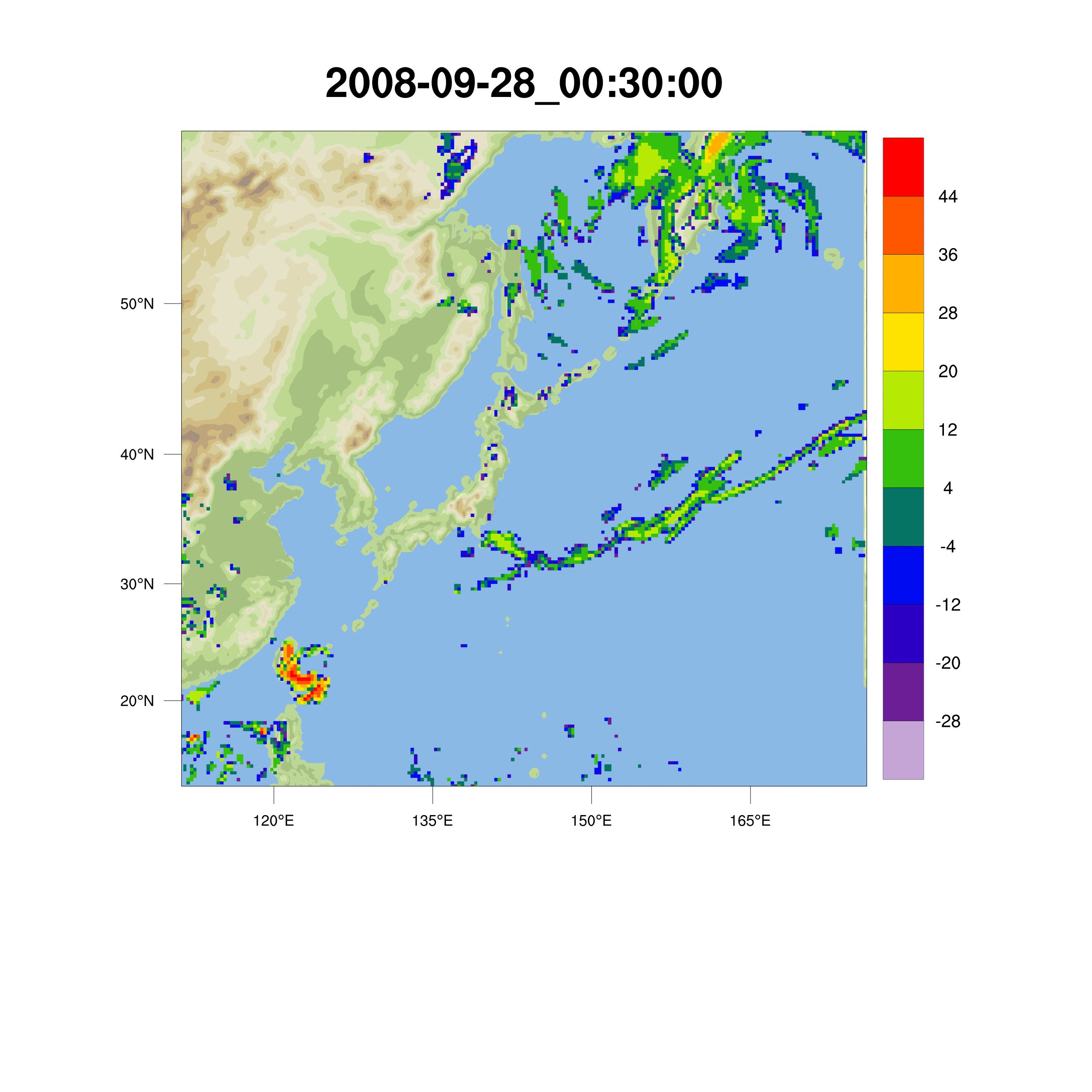
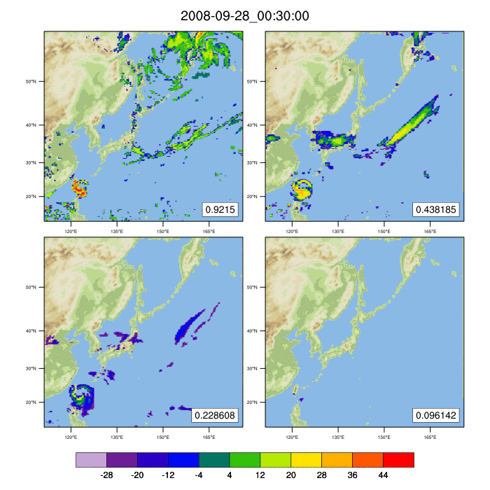
The animation is filled contours of WRF reflectivity across time, overlaid on a WRF terrain plot. The terrain plot is the same for each iteration, while the reflectivity plot and the title change for each time step.

animate_3_1.ncl - this script shows the traditional and "easy" way to do this, but also potentially slower, by calling gsn_csm_contour, gsn_csm_contour_map, and overlay each time in the loop.

animate_3_2.ncl - this script shows how to speed this up a little by reusing the terrain plot.

animate_3_3.ncl - this script shows how to speed this up even more, by using setvalues to simply change the data and the title.

The timings on a Mac system were as follows:

"animate_3_1.ncl" - 98.34 seconds
"animate_3_2.ncl" - 92.83 seconds
"animate_3_3.ncl" - 84.85 seconds

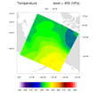
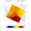
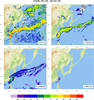
Click on thumbnail image for an animation

The animation was created by generating a series of PNG images, and then calling:

convert animate*.00*png animate_3.gif

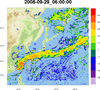
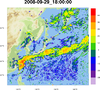
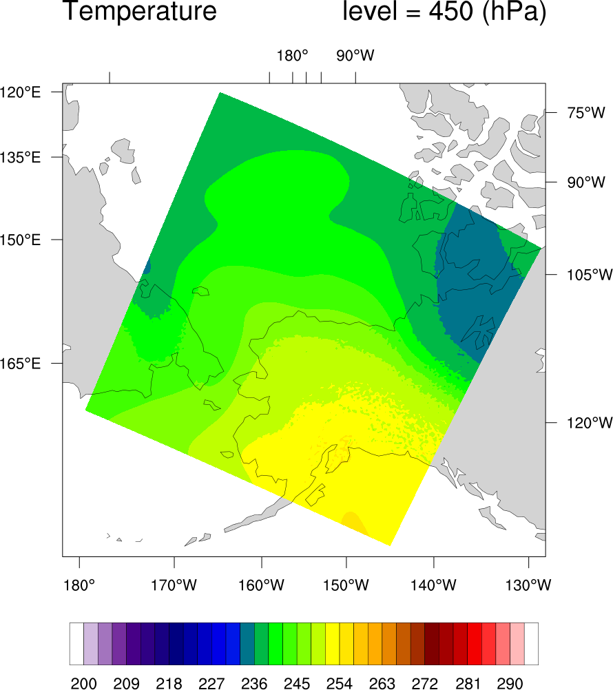
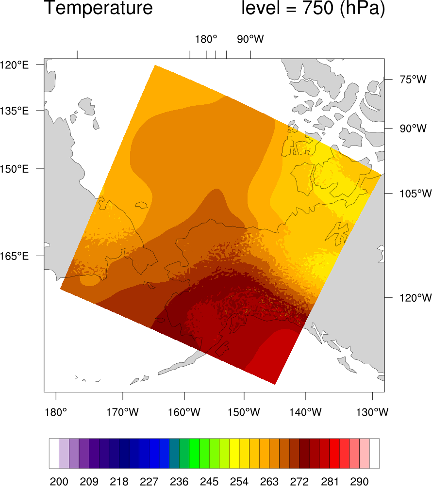
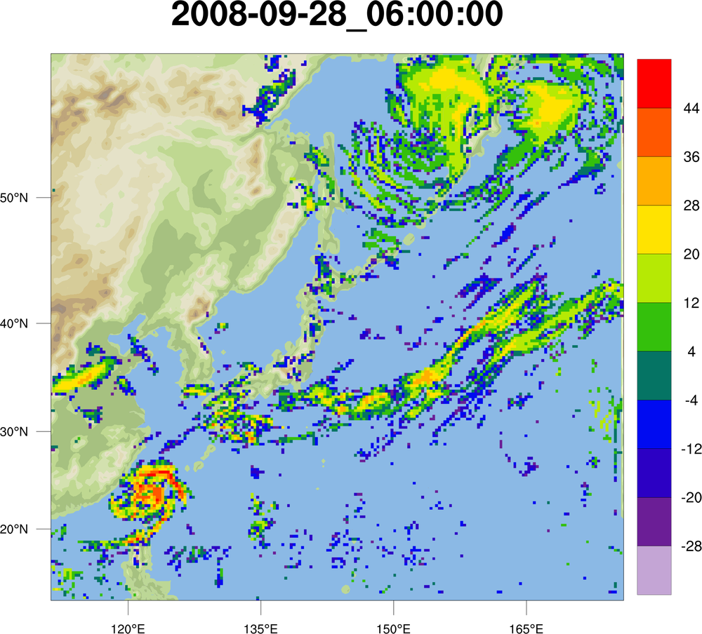
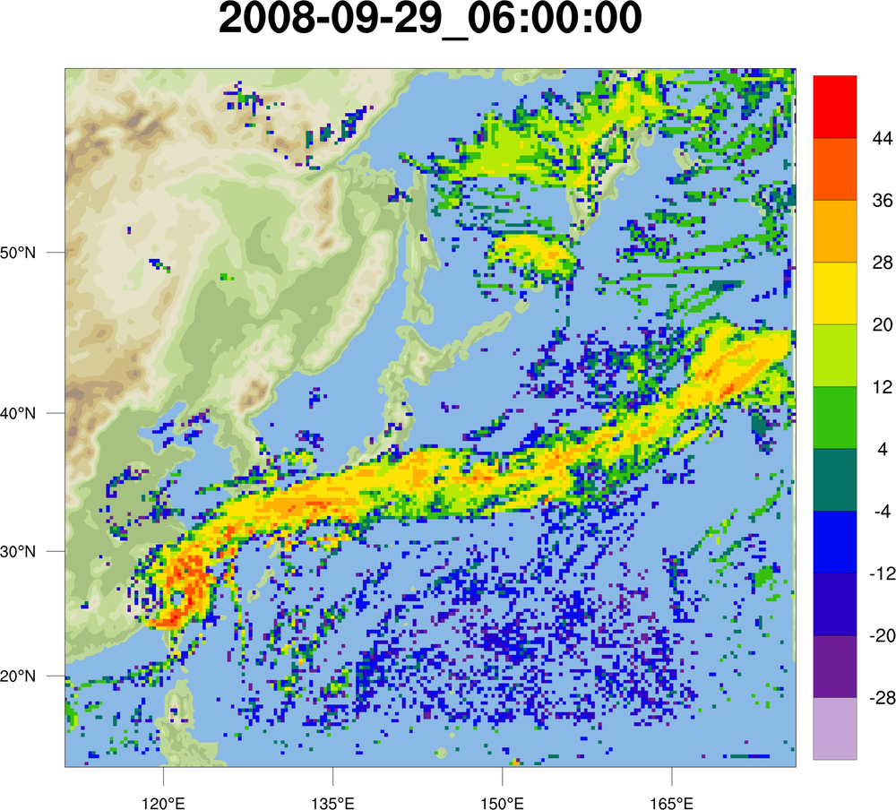
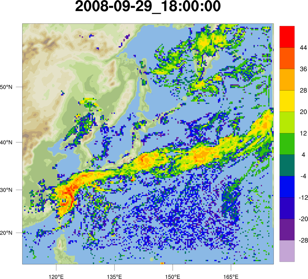
animate_4_1.ncl /
animate_4_2.ncl:

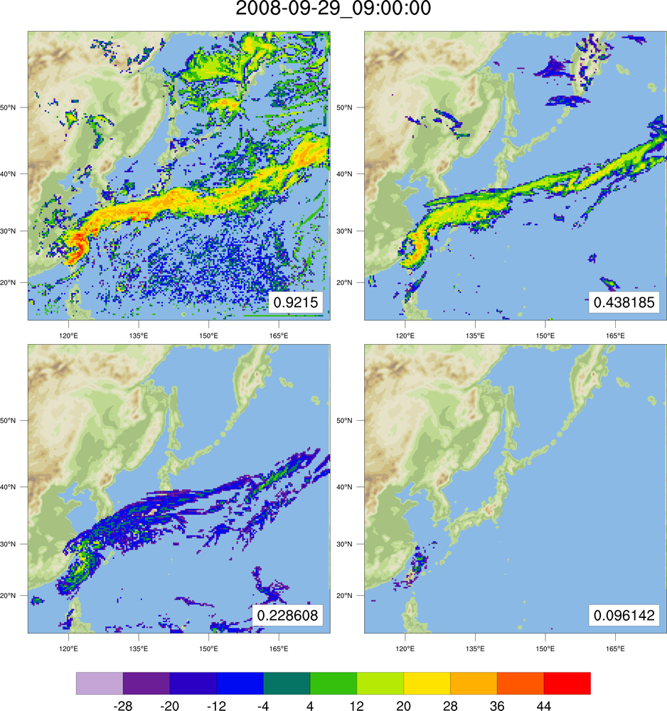
This example shows two ways to create a 97-frame 4-panel animation in NCL, with tips on how to speed things up. It's based on the script from the previous example, except now four plots are animated per page.

The animation is filled contours of WRF reflectivity (across time and four selected level indexes) overlaid on a WRF terrain plot. The terrain plot is the same for each iteration, while the reflectivity plots change for each time and level.

animate_4_1.ncl - this script shows the traditional and "easy" way to do this, but also potentially slower, by calling gsn_csm_contour, gsn_csm_contour_map, and overlay each time in the loop.

animate_4_2.ncl - this script shows how to speed this up a little by using "setvalues" on existing reflectivity plots to simply change the data.

The timings on a Mac system were as follows:

"animate_4_1.ncl" - 163.0 seconds
"animate_4_2.ncl" - 129.8 seconds

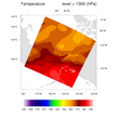
Click on thumbnail image for an animation

The animation was created by generating a series of PNG images, and then calling:

convert animate*.00*png animate_4.gif