NCL Graphics: CloudSat: Cloud Vertical Structure

CloudSat is a satellite mission designed to measure the vertical structure of clouds from space. The radar data produces detailed images of cloud structures which will contribute to a better understanding of clouds and climate.

CloudSat along with CALIPSO, Aqua, PARASOL, and Aura form a satellite constellation known as the A-Train. The satellites fly in a nearly circular orbit with an equatorial altitude of approximately 705 km. The orbit is sun-synchronous, maintaining a roughly fixed angle between the orbital plane and the mean solar meridian. CloudSat maintains a close formation with Aqua and a particularly close formation with CALIPSO, providing near-simultaneous and collocated observations with the instruments on these two platforms. (Note that PARASOL was maneuvered to leave its position inside the A-Train on December 2, 2009.)

The CFMIP-OBS (Cloud Feedback Model Intercomparison Program) has designed a protocol to evaluate clouds in climate and weather prediction models based on satellite observations.

The 2B-CLDCLASS documentation is NCL, Matlab, IDL and Python examples which includes both scripts and the created graphical images. They also provide NCL specific comments.

This site is updated so CloudSat examples may be added in the future. Please check.

2B-CLDCLASS

Source: http://www.cloudsat.cira.colostate.edu/ICD/2B-CLDCLASS/2B-CLDCLASS_PDICD_5.0.pdf
 
           Table 5. File Specification for 16-Bit cloud scenario

                       16 Bit Cloud Scenario File Specification
Bit Field              Description Key            Result
   0                   Cloud scenario flag        0 = not determined 
                                                  1 = determined
                       -------------------
  1-4                  Cloud scenario             0000 = No cloud
                                                  0001 = cirrus
                                                  0010 = Altostratus
                                                  0011 = Altocumulus
                                                  0100 = St
                                                  0101 = Sc
                                                  0110 = Cumulus
                                                  0111 = Ns
                                                  1000 = Deep Convection
                       -------------------
  5-6                  Land/sea flag              00 = no specific
                                                  01 = land
                                                  10 = sea
                                                  11= snow (?)
                       -------------------
  7-8                  Latitude flag              00 = tropical
                                                  01 = midlatitude
                                                  10 = polar
                       -------------------
  9-10                 Algorithm flag             00 = radar only
                                                  01 = combined radar and MODIS
                       -------------------
 11-12                 Quality flag               00 = not very confident
                                                  01 = confident
                       -------------------
 13-14                 Precipitation flag         00 = no precipitation
                                                  01 = liquid precipitation
                                                  10 = solid precipitation
                                                  11 = possible drizzle
                       -------------------
  15                   Spare

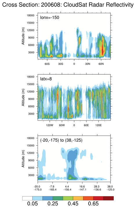
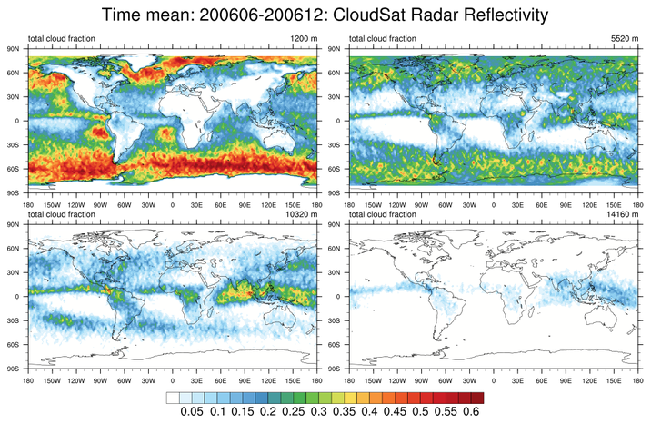
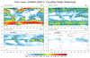
cloudsat_1.ncl: (1) Average "CloudSat Radar Reflectivity" over the period 200606-200612 at user specified levels; (2) Radar reflectivity in the vertical at user specified (lat,lon) locations; (3) User specified cross sections. The last cross section uses linint2_points_Wrap to interpolate to a series of arbitrary points. The gc_latlon is used to generate the points on a great circle path.

The file used in this example was obtained from: ftp://ftp.climserv.ipsl.polytechnique.fr/cfmip/CloudSat/CloudSat_Reflectivity/cfadDbze94_200606-200612.nc

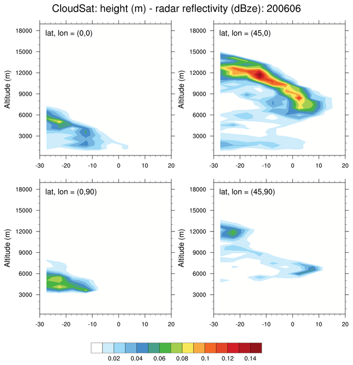
cloudsat_2.ncl:

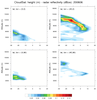
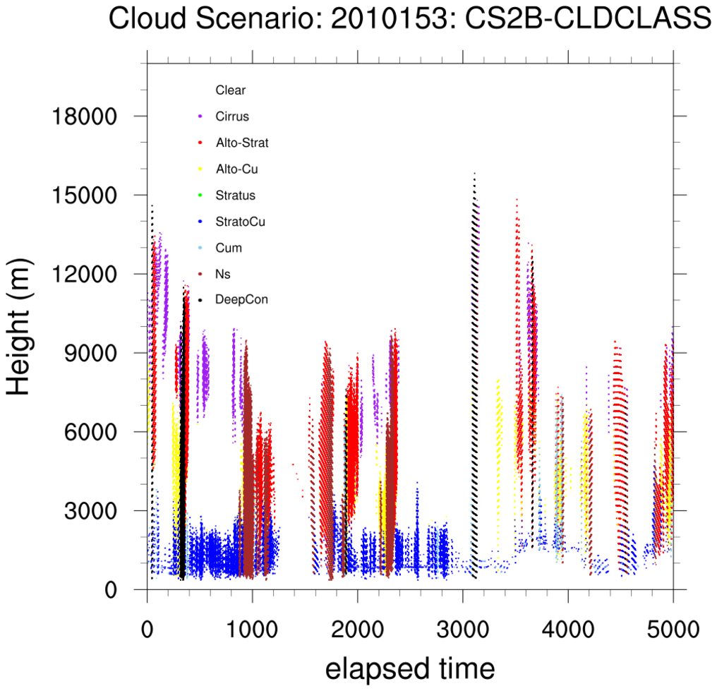
This file is CLOUDSAT 2B-CLDCLASS. The variable being plotted cloud_scenario is "Algorithm outputs (cloud type and different flags) are combined into a 16 bit cloud_scenario." Hence, the variable of type 'short' must be unpacked using dim_gbits.

The ncl_filedump command line operator was used to examine the file prior to use. The generic .hdf extension 'hides' the fact that this is a HDF-EOS file. Further, the file contains a satellite swath (GROUP=SwathStructure).

ncl_filedump 2010153190053_21792_CS_2B-CLDCLASS_GRANULE_P_R04_E03.hdf | less

[snip]

filename:       2010153190053_21792_CS_2B-CLDCLASS_GRANULE_P_R04_E03

   file global attributes:
      HDFEOSVersion : HDFEOS_V2.5
      StructMetadata_0 : GROUP=SwathStructure
[SNIP]

Since this is a HDF-EOS file, the file is read with a ".he2" or ".hdfeos" extension in the addfile function. This tells NCL to read the file with both the standard HDF and HDF-EOS read software. NCL merges the information so user have one unified view of the file.

This script reads and unpacks the appropriate variables. A color 'contour map' displays the information.

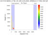
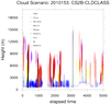cloudsat_poly_2.ncl:

Similar to cloudsat_2 except that individual polymarkers are used to show every value. In practice the figure associated with cloudsat_2 can be considered a low-pass verion of the cloudsat_poly_2.

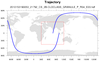
cloudsat_3.ncl:

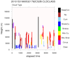
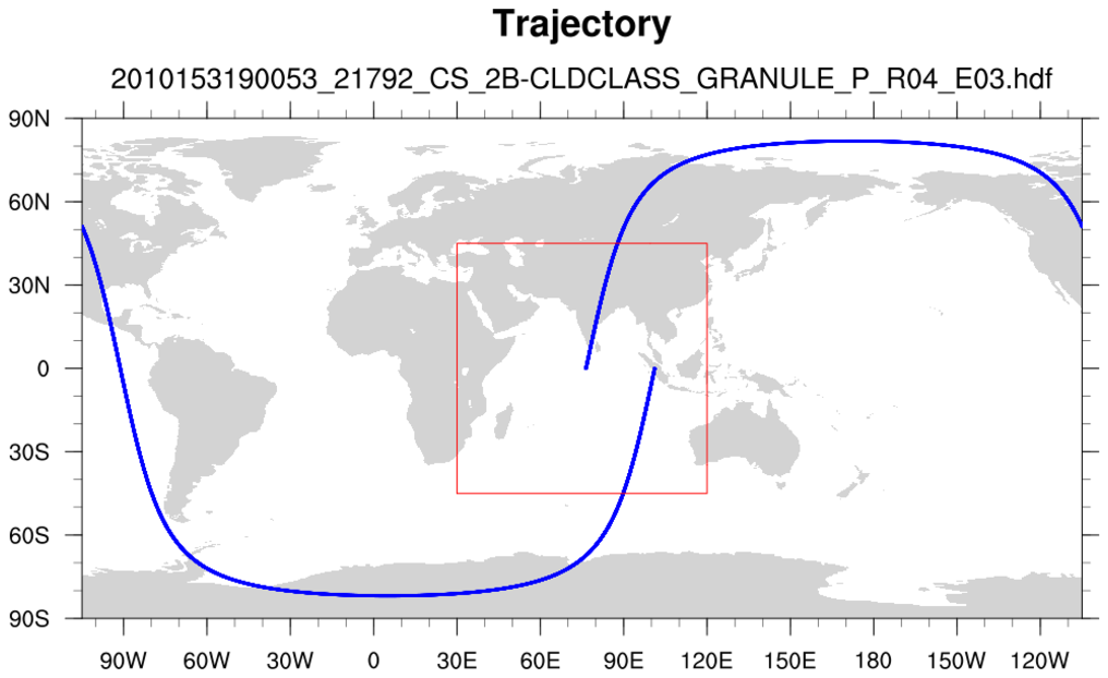
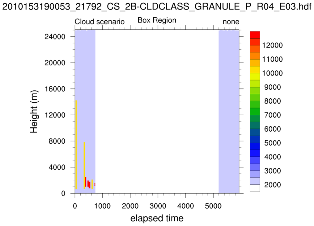
See opening statement for Example 2.

Same data file as Example 2. Plot the total trajectory. Specify a region of interest and plot an outline of the area. Then plot only data which occurred in the region of interest. Manually specify a finer contour interval. NOTE: The satellite is within the specified region at the beginning and end of the time interval.