The primary purpose of the Penman-Monteith method is to calculate the loss of water from land surfaces due to evaporation.
NCL Home>
Application examples>
Data Analysis ||
Data files for some examples

 fao56_1.ncl:
Example 1: Using data generated by the CESM-CLM component,
this example illustrates the standardized approach
to computing the Penman-Monteith reference evapotranspiration via FAO-56 methodology:
(refevt_penman_fao56).
fao56_1.ncl:
Example 1: Using data generated by the CESM-CLM component,
this example illustrates the standardized approach
to computing the Penman-Monteith reference evapotranspiration via FAO-56 methodology:
(refevt_penman_fao56).
 fao56_1a.ncl: Example 1a: Same as Example 1 but use the "tall"
hypothetical reference crop coefficients specified by the ASCE-ET (American Society of Civil Engineering)
for a hypothetical "tall" crop (cnumer=1600 and cdenom=0.38).
fao56_1a.ncl: Example 1a: Same as Example 1 but use the "tall"
hypothetical reference crop coefficients specified by the ASCE-ET (American Society of Civil Engineering)
for a hypothetical "tall" crop (cnumer=1600 and cdenom=0.38).
 fao56_2.ncl: Example 2:
Use the radext_fao56 and daylight_fao56
to calculate the extraterrestrial radiation and maximum number of daylight hours
as described in FAO 56.
fao56_2.ncl: Example 2:
Use the radext_fao56 and daylight_fao56
to calculate the extraterrestrial radiation and maximum number of daylight hours
as described in FAO 56.
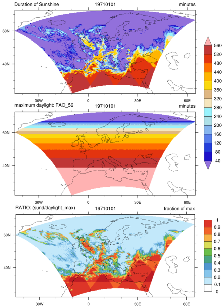
 fao56_3.ncl: Example 3:
Use daylight_fao56 to calculate the maximum daylight duration
as described in FAO 56.
Compare the theoretical maximum daylight with the modeled ('observed') sunshine duration
for a particular day by computing the ratio.
fao56_3.ncl: Example 3:
Use daylight_fao56 to calculate the maximum daylight duration
as described in FAO 56.
Compare the theoretical maximum daylight with the modeled ('observed') sunshine duration
for a particular day by computing the ratio.
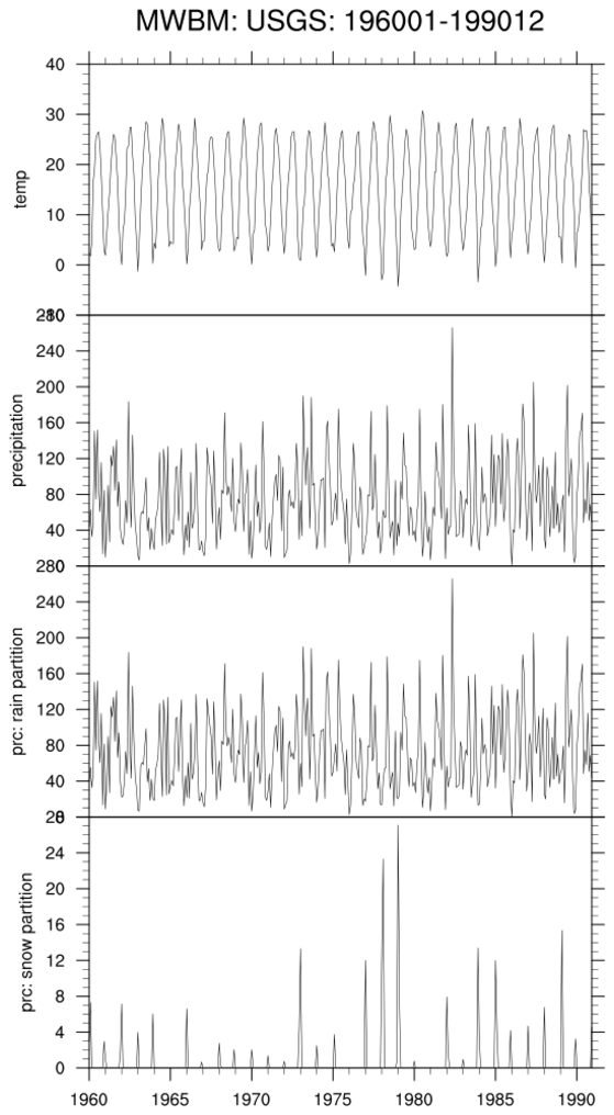
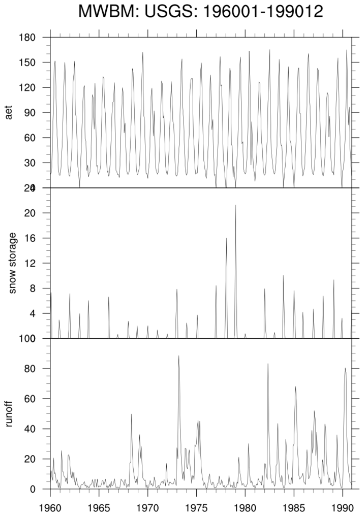
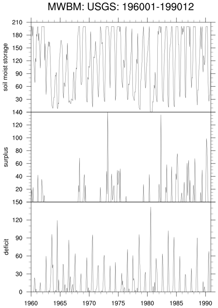
 mwbm_1.ncl:
Read the ascii text file
(here: MWBM_USGS.input_file.txt) used by McGabe and Markstrom (2007).
Use refevt_hamon to calculate the
potential evapotranspiration. Print and plot selected hydrologic components.
mwbm_1.ncl:
Read the ascii text file
(here: MWBM_USGS.input_file.txt) used by McGabe and Markstrom (2007).
Use refevt_hamon to calculate the
potential evapotranspiration. Print and plot selected hydrologic components.
 mwbm_2.ncl:
Same as Example 1 but read observed monthly data for Boulder, CO [USA]. The data are
contained within netCDF files. Print and plot selected hydrologic components.
mwbm_2.ncl:
Same as Example 1 but read observed monthly data for Boulder, CO [USA]. The data are
contained within netCDF files. Print and plot selected hydrologic components.

 mwbm_3.ncl:
Read CESM time series from a 'control' experiment at user specified grid locations.
Change units to mm/month. Print and plot selected hydrologic components.
mwbm_3.ncl:
Read CESM time series from a 'control' experiment at user specified grid locations.
Change units to mm/month. Print and plot selected hydrologic components.

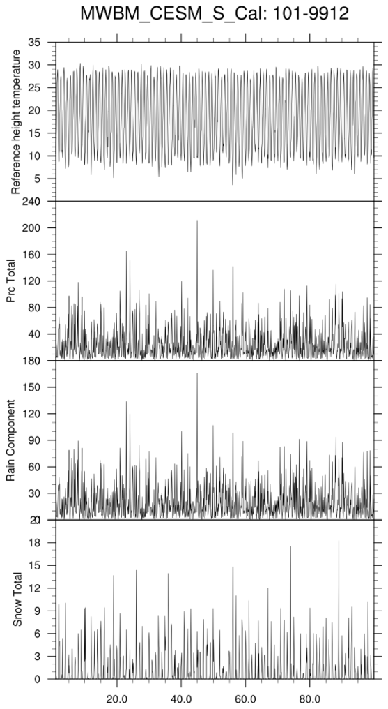
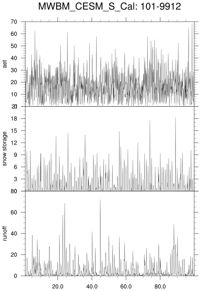
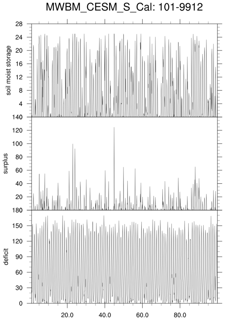
 mwbm_4.ncl:
Read CESM time series data from a grid section over Southern California.
Use landsea_mask to create a mask
so that ocean locations are not used. Average all hydrolocal quantities for the grid section.
Print and plot averaged hydrologic components.
mwbm_4.ncl:
Read CESM time series data from a grid section over Southern California.
Use landsea_mask to create a mask
so that ocean locations are not used. Average all hydrolocal quantities for the grid section.
Print and plot averaged hydrologic components.
Example pages containing: tips | resources | functions/procedures
Crop: Evapotranspiration: FAO 56, Penman-Monteith, Monthly Water Balance Model
The Food and Agriculture Organization (FAO) Irrigation and Drainage
paper 56 document
provides the definitive standardized methodology for deriving estimates
of reference evapotranspiration (aka, ET0) for a hypothetical "short" crop.
Subsequently, the ASCE-ET (American Society of Civil Engineering) created additional parameters
for a hypothetical "tall" crop (full-cover alfalfa). See Example 1a.
NCL has implemented virtually all the FAO referenced equations into a
library of functions
which calculate many of the terms required to estimate evapotranspirtation.
The "crop" function category is documented
here.
The following [1]-[3] descriptions are quoted from WikiPedia:
- Evapotranspiration (ET) is the sum of evaporation and plant transpiration from the Earth's land and ocean surface to the atmosphere. Evaporation accounts for the movement of water to the air from sources such as the soil, canopy interception, and waterbodies. Transpiration accounts for the movement of water within a plant and the subsequent loss of water as vapor through stomata in its leaves. Evapotranspiration is an important part of the water cycle.
- Reference evapotranspiration (ET0), sometimes incorrectly referred to as potential ET, is a representation of the environmental demand for evapotranspiration and represents the evapotranspiration rate of a short green crop (grass), completely shading the ground, of uniform height and with adequate water status in the soil profile. It is a reflection of the energy available to evaporate water, and of the wind available to transport the water vapour from the ground up into the lower atmosphere. Actual evapotranspiration is said to equal reference evapotranspiration when there is ample water. Some US states utilize a full cover alfalfa reference crop that is 0.5 m in height, rather than the short green grass reference, due to the higher value of ET from the alfalfa reference.
- Potential evaporation or potential evapotranspiration (PET) is defined as the amount of evaporation that would occur if a sufficient water source were available. If the actual evapotranspiration is considered the net result of atmospheric demand for moisture from a surface and the ability of the surface to supply moisture, then PET is a measure of the demand side. Surface and air temperatures, insolation, and wind all affect this. A dryland is a place where annual potential evaporation exceeds annual precipitation.
- A brief description of the difference between potential evapotranspiration (PET) and reference evapotranspiration(ETo) is
the Irman and Hamon (2003/2014) reference. It is available here.
- A brief description of the significance of evapotranspiration and its relationship to drought and the hydrological cycle is Hanson (1991). It is available here.
References: FAO-56: Penman-Monteith
  Richard G. Allen, Luis S. Pereira, Dirk Raes, Martin Smith (1998)
  Crop Evapotranspiration - Guidelines for Computing Crop Water Requirements
       FAO Irrigation and drainage paper 56. Rome, Italy:
  Food and Agriculture Organization of the United Nations.
  WWW: http://www.fao.org/docrep/X0490E/x0490e00.htm
  In particular: Chapter 3 (Meteorological Data) & Chapter 4 (Determination of ET0)

  --------------------------

  Zotarelli, L. et al (2013)
  Step by Step Calculation of the Penman-Monteith Evapotranspiration (FAO-56 Method)
  WWW: http://edis.ifas.ufl.edu/pdffiles/ae/ae45900.pdf

  --------------------------

  Tools for Agro-Meteorology and Biophysical Modelling
  http://agsys.cra-cin.it/tools/EvapoTranspiration/help/
          Click Equations, Evapotranspirations Equations, Supporting Equations
References: Actual, Reference and Potential Evapotranspiration
Pidwirny, M. (2006). Actual and Potential Evapotranspiration Fundamentals of Physical Geography, 2nd Edition. WWW: http://www.physicalgeography.net/fundamentals/8j.html Irmak, S. and D.Z. Haman (2003; original; 2014: most recent) Evapotranspiration: Potential or Reference? WWW: https://edis.ifas.ufl.edu/ae256 Agricultural and Biological Engineering Department, UF/IFAS Extension.References: ASCE Standardized Reference Evapotranspiration Equation
Jensen, M.E., R.D. Burman, and R.G. Allen. (1990) Evapotranspiration and Irrigation Water Requirements ASCE Manuals and Reports on Engineering Practice No. 70 Am. Soc. Civil Engr., New York, NY. 332 pp.
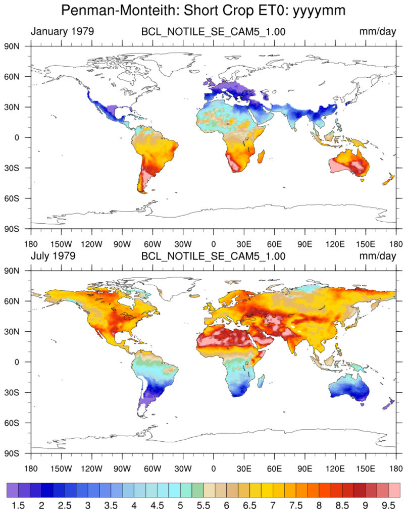
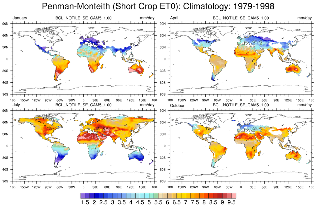
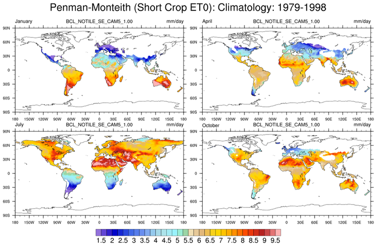
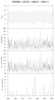
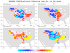
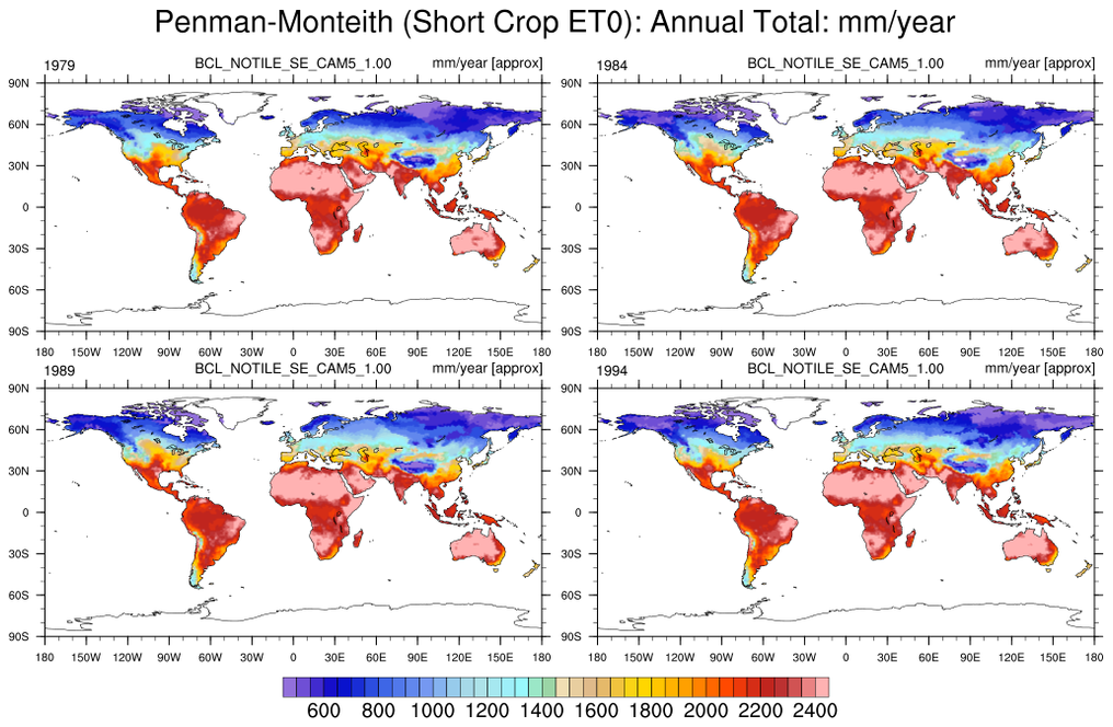 fao56_1.ncl:
Example 1: Using data generated by the CESM-CLM component,
this example illustrates the standardized approach
to computing the Penman-Monteith reference evapotranspiration via FAO-56 methodology:
(refevt_penman_fao56).
fao56_1.ncl:
Example 1: Using data generated by the CESM-CLM component,
this example illustrates the standardized approach
to computing the Penman-Monteith reference evapotranspiration via FAO-56 methodology:
(refevt_penman_fao56).
This example uses the FAO-56 recommended:
- albedo=0.23: This albedo is not the atmospheric or land surface albedo. Rather,
the albedo refers to light reflected by the crop leaf surface ('leaf_albedo').
- cnumer=900 and cdenom=0.34. These are the FAO-56 values appropriate for the hypothetical (short) reference crop. They are appropriate for day and month estimates. To apply to hourly data use (cnumer=37.5 [=900.0/24])
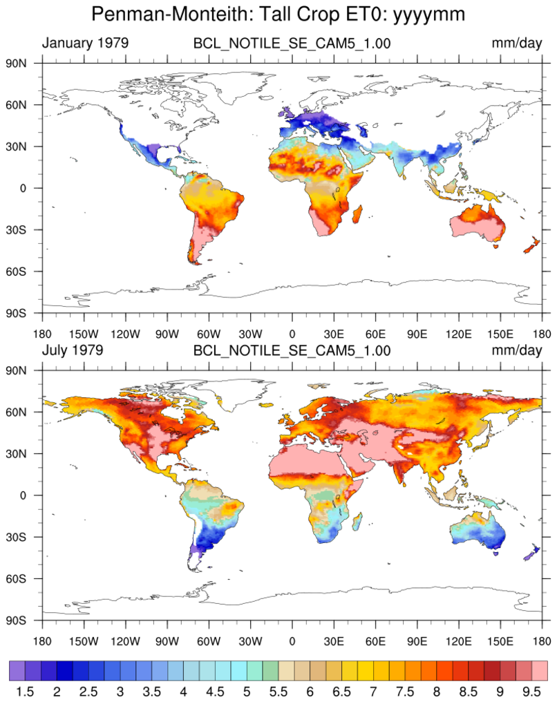
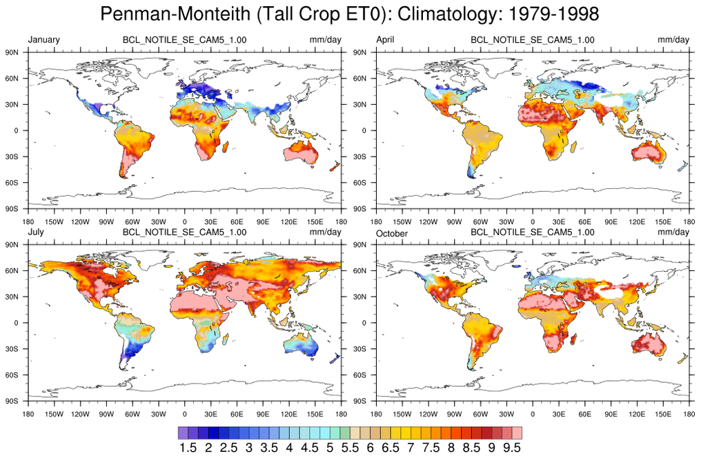
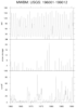
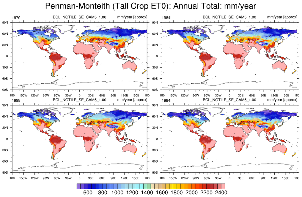 fao56_1a.ncl: Example 1a: Same as Example 1 but use the "tall"
hypothetical reference crop coefficients specified by the ASCE-ET (American Society of Civil Engineering)
for a hypothetical "tall" crop (cnumer=1600 and cdenom=0.38).
fao56_1a.ncl: Example 1a: Same as Example 1 but use the "tall"
hypothetical reference crop coefficients specified by the ASCE-ET (American Society of Civil Engineering)
for a hypothetical "tall" crop (cnumer=1600 and cdenom=0.38).
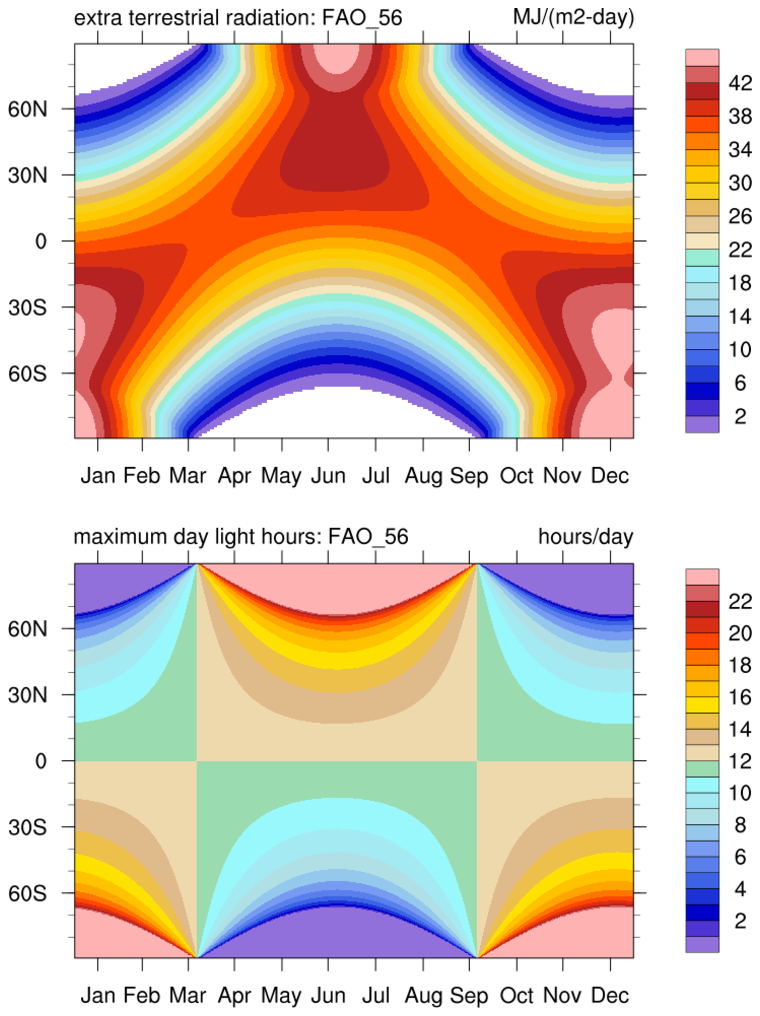 fao56_2.ncl: Example 2:
Use the radext_fao56 and daylight_fao56
to calculate the extraterrestrial radiation and maximum number of daylight hours
as described in FAO 56.
fao56_2.ncl: Example 2:
Use the radext_fao56 and daylight_fao56
to calculate the extraterrestrial radiation and maximum number of daylight hours
as described in FAO 56.
NOTE_1: The assumptions used to derive the 'simple' equations used by FAO-56 are less appropriate for latitudes poleward of (say) 55-60 degrees.
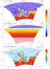
NOTE_2: Printed values (W/m2) at selected latitudes for each day of the year are here. These are from Example 3 at radext_fao56.
NOTE_3: If the user wishes all returned _FillValue to be set to zero (0.0), then after the radext_fao56 function use the where and ismissing functions to set all _FillValue to zero. Specifically:
  radext = radext_fao56(jday, lat, ounit)
  radext = where(ismissing(radext), 0, radext)  ; set all _FillValue = 0.0
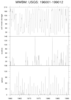
 fao56_3.ncl: Example 3:
Use daylight_fao56 to calculate the maximum daylight duration
as described in FAO 56.
Compare the theoretical maximum daylight with the modeled ('observed') sunshine duration
for a particular day by computing the ratio.
fao56_3.ncl: Example 3:
Use daylight_fao56 to calculate the maximum daylight duration
as described in FAO 56.
Compare the theoretical maximum daylight with the modeled ('observed') sunshine duration
for a particular day by computing the ratio.
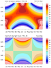
Use two different types of label bars: (a) triangle ends and (b) fixed ends with no outer boxes.
Monthly Water-Balance Model The McGabe and Markstrom (2007) Monthly Water Balance Model (MWBM)) allocates monthly water to various components of the hydrologic system. A visual diagram of the MWBM is contained within the McCabe and Markstrom (2007) reference. Also: here.
NCL's mwbm_driver differs from the McGabe and Markstrom (2007) implementation. It allows the user to input monthly pet and snow total while the USGS implementation calculates these variables internally. An advantage of the mwbm_driver approach is that users can precompute pet using one of NCL's suite of 'PET' functions (see below). Further, if available, the user can explicitly input the observed snow (liquid equivalent) rather than use empirical estimates.
Multiple hydrologic variables are returned, including:
- Actual EvapoTranspiration (AET): Actual amount of evapotranspiration that occurs,
- Direct RunOff (DRO): Water that flows over the ground surface directly into streams, rivers, or lakes.
- RunOff (RO) [Surplus runoff]: Precipitation that did not get (infiltrated) absorbed into the soil or did not evaporate.
- Soil Moisture Storage (SMS): Water that is held in the spaces between soil particles. Commonly: Surface soil moisture is the water that is in the upper 10 cm of soil, whereas root zone soil moisture is the water that is available to plants, which is generally considered to be in the upper 200 cm of soil. Soil moisture levels rise when there is sufficient rainfall to exceed losses to evapotranspiration and drainage to streams and groundwater. Often, they are depleted during the summer when evapotranspiration rates are high.
- Snow Melt (SM): surface runoff produced from melting snow.
What is the difference between water holding capacity and field capacity? Available water is the difference between field capacity which is the maximum amount of water the soil can hold and wilting point where the plant can no longer extract water from the soil. Water holding capacity is the total amount of water a soil can hold at field capacity.
See the mwbm_*.ncl examples for various methods of application..
Primary Reference:
   A Monthly Water-Balance Model Driven By a Graphical User Interface
   Gregory J. McCabe and Steven L. Markstrom
   U.S. Geological Survey; U.S. Department of the Interio
   Open-File Report 2007–1088
Other References:
   The U.S. Geological Survey Monthly Water Balance Model Futures Portal
   Bock, A.R., Hay, L.E., Markstrom, S.L., Emmerich, Chris, and Talbert, Marian (2017)
   U.S. Geological Survey Open-File Report 2016-1212, 21 p.

   Parameter regionalization of a monthly water balance model for
              the conterminous United States
   Bock, A.R. et al
   Hydrol. Earth Syst. Sci., 20, 2861-2876, 2016

   Comparison of Performance of Twelve Monthly Water Balance Models
             in Different Climatic Catchments of China
   Peng Bai, Xiaomang Liu, Kang Liang, Changming Liu
   Journal of Hydrology
   Volume 529, Part 3, October 2015, Pages 1030-1040
The mwbm_driver script is available here.
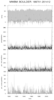
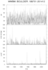
 mwbm_1.ncl:
Read the ascii text file
(here: MWBM_USGS.input_file.txt) used by McGabe and Markstrom (2007).
Use refevt_hamon to calculate the
potential evapotranspiration. Print and plot selected hydrologic components.
mwbm_1.ncl:
Read the ascii text file
(here: MWBM_USGS.input_file.txt) used by McGabe and Markstrom (2007).
Use refevt_hamon to calculate the
potential evapotranspiration. Print and plot selected hydrologic components.


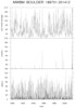
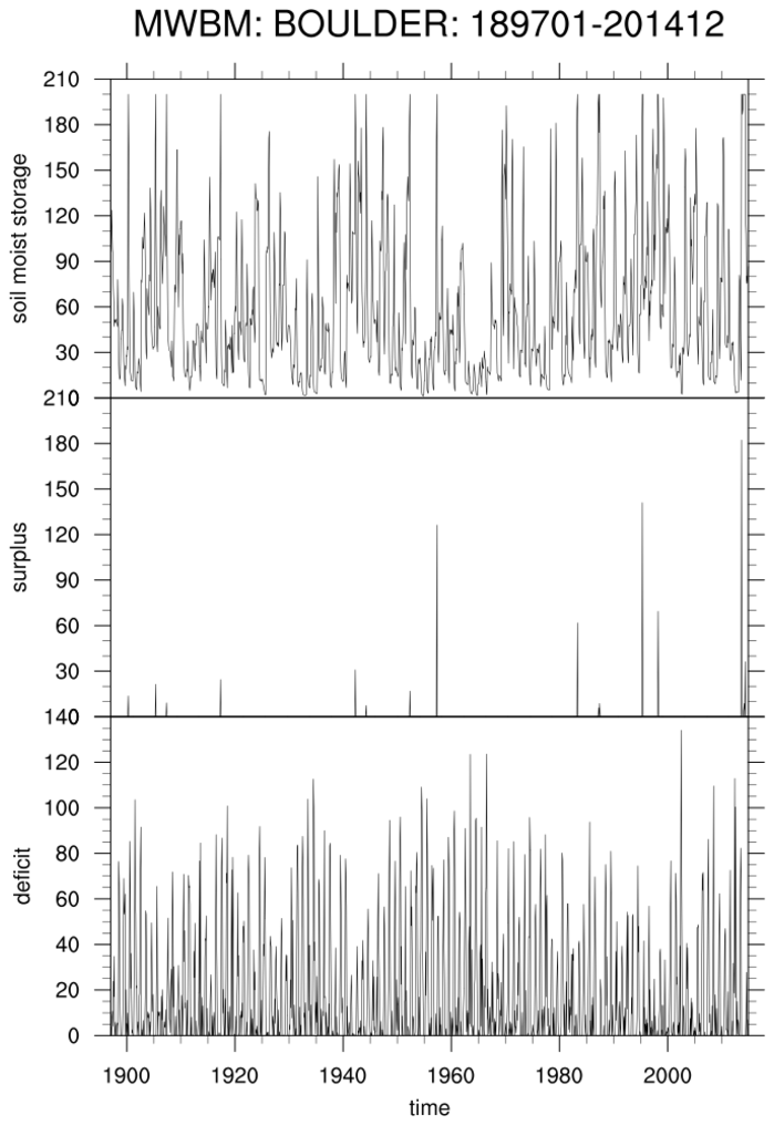 mwbm_2.ncl:
Same as Example 1 but read observed monthly data for Boulder, CO [USA]. The data are
contained within netCDF files. Print and plot selected hydrologic components.
mwbm_2.ncl:
Same as Example 1 but read observed monthly data for Boulder, CO [USA]. The data are
contained within netCDF files. Print and plot selected hydrologic components.
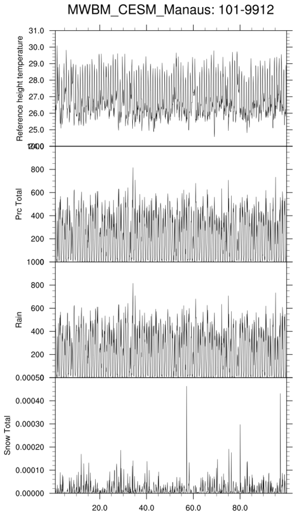
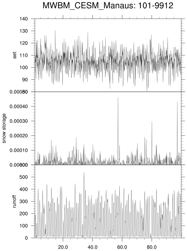
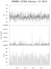
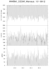
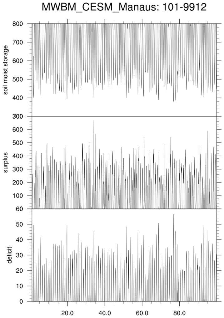 mwbm_3.ncl:
Read CESM time series from a 'control' experiment at user specified grid locations.
Change units to mm/month. Print and plot selected hydrologic components.
mwbm_3.ncl:
Read CESM time series from a 'control' experiment at user specified grid locations.
Change units to mm/month. Print and plot selected hydrologic components.
The example uses just one location corresponding to Manaus, Brazil. However, there can be multiple locations specified.
 mwbm_4.ncl:
Read CESM time series data from a grid section over Southern California.
Use landsea_mask to create a mask
so that ocean locations are not used. Average all hydrolocal quantities for the grid section.
Print and plot averaged hydrologic components.
mwbm_4.ncl:
Read CESM time series data from a grid section over Southern California.
Use landsea_mask to create a mask
so that ocean locations are not used. Average all hydrolocal quantities for the grid section.
Print and plot averaged hydrologic components.
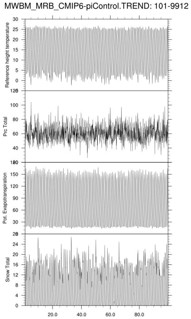
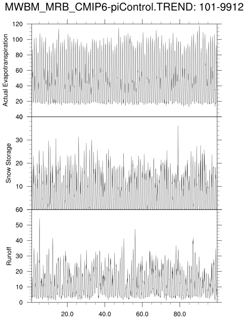
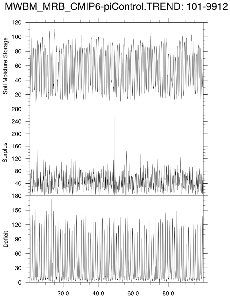
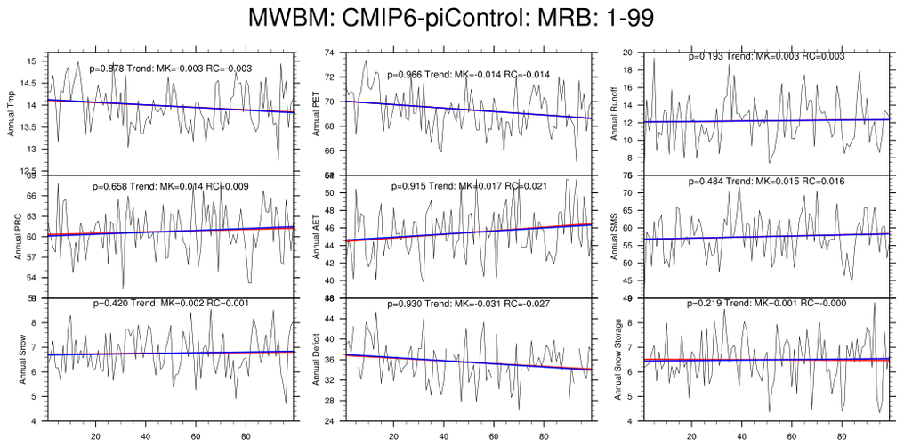
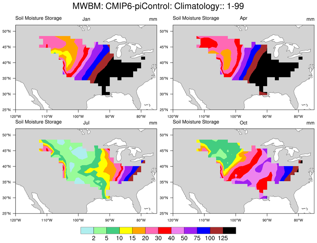

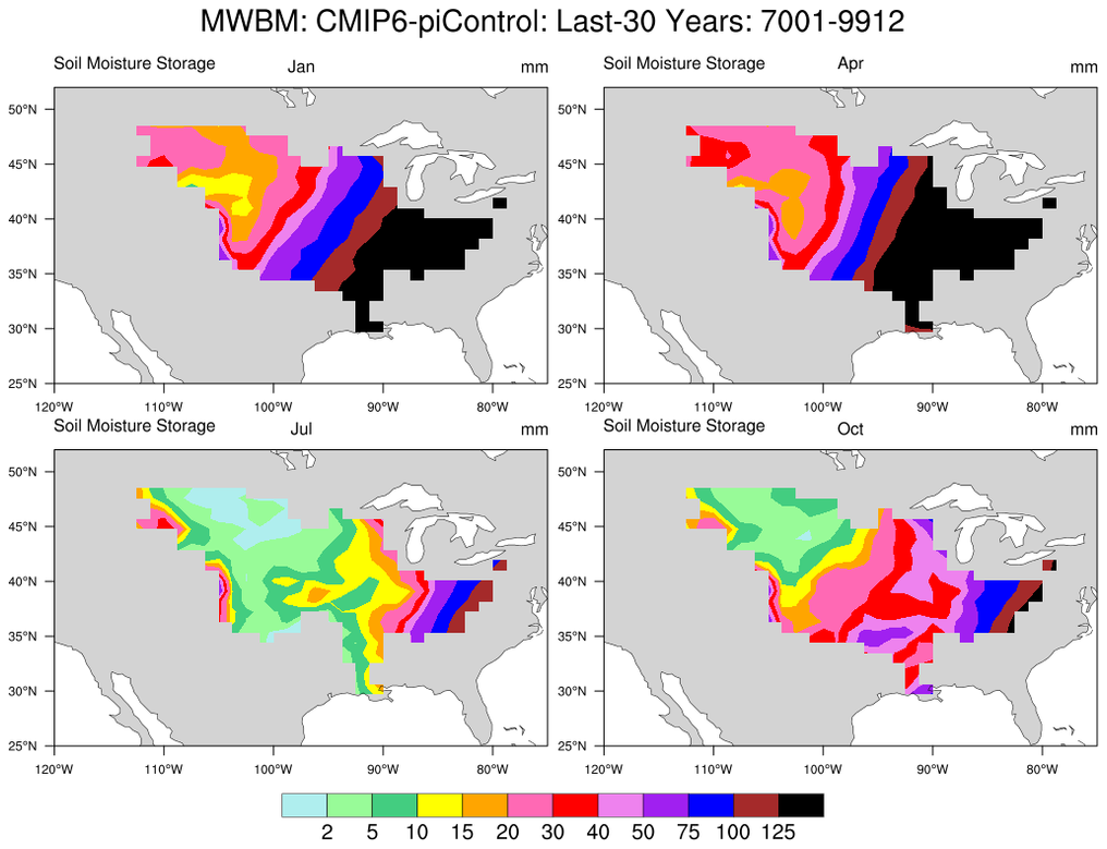
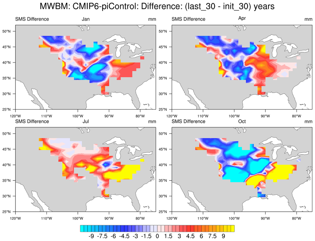
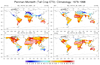
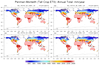
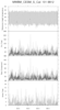
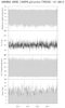
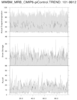
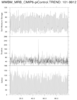
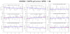
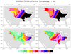
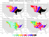
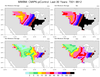
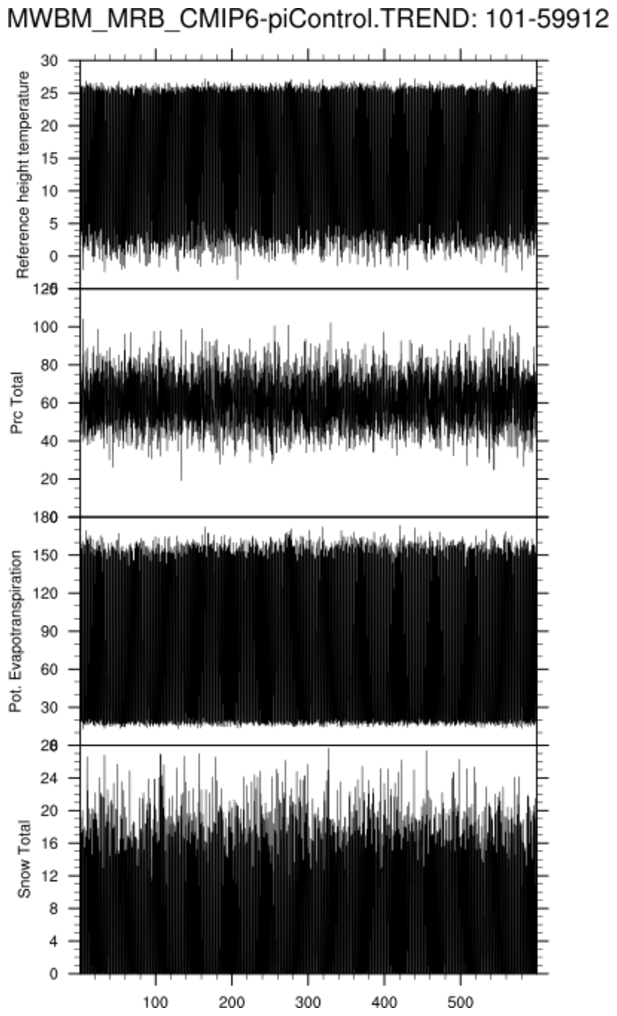
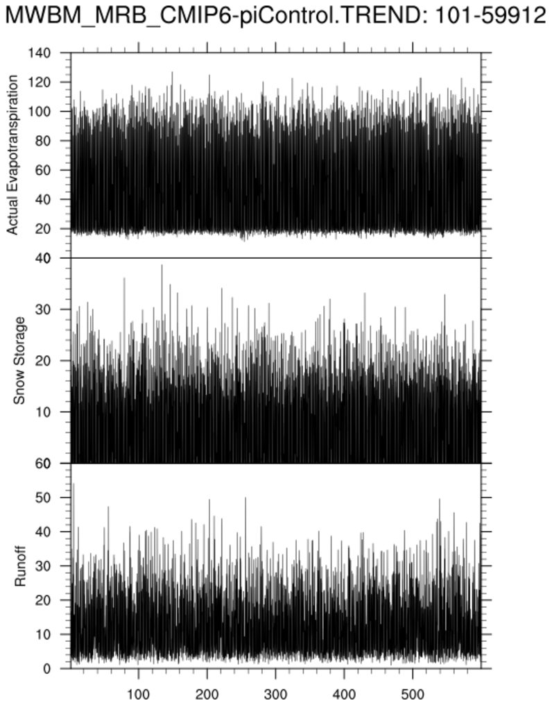
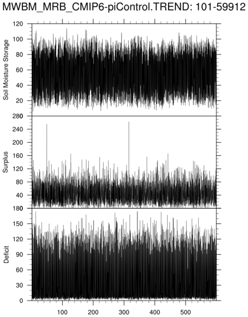
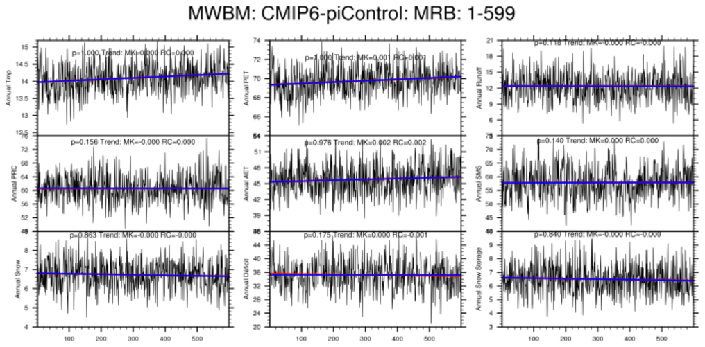
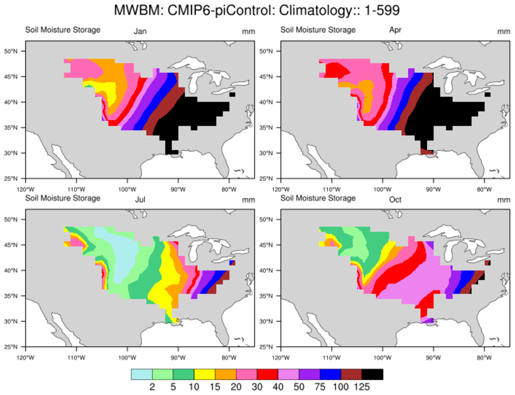
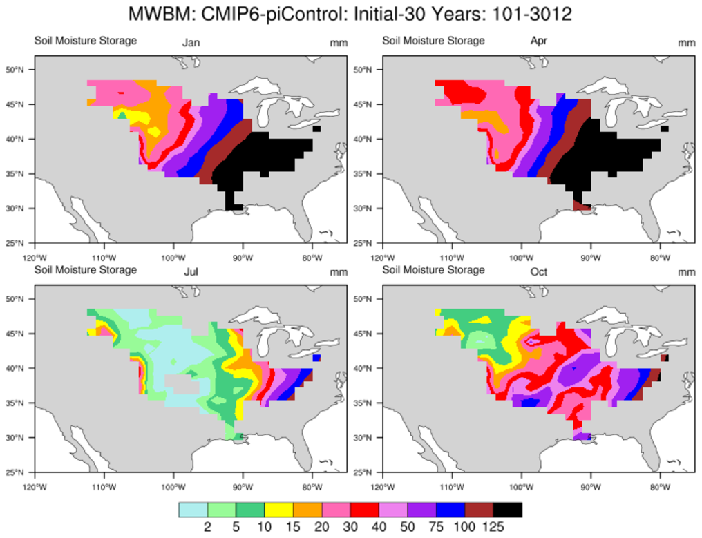
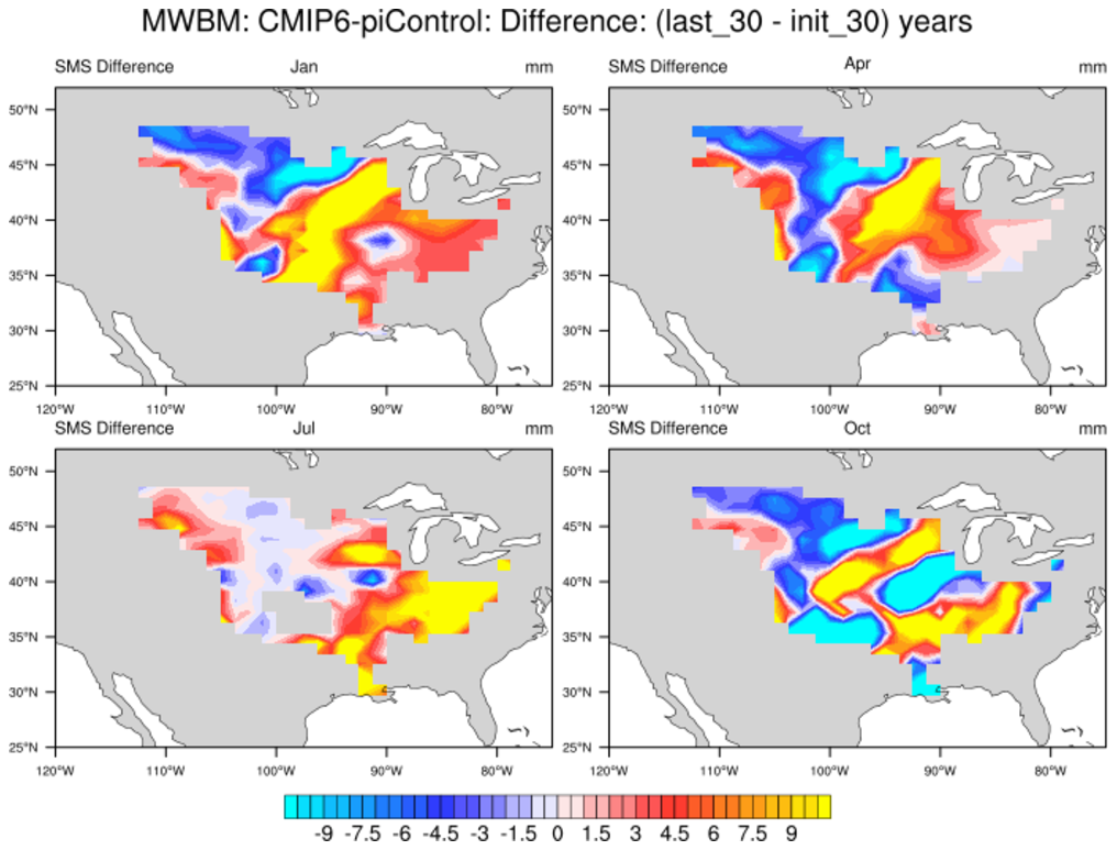
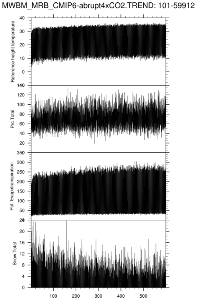
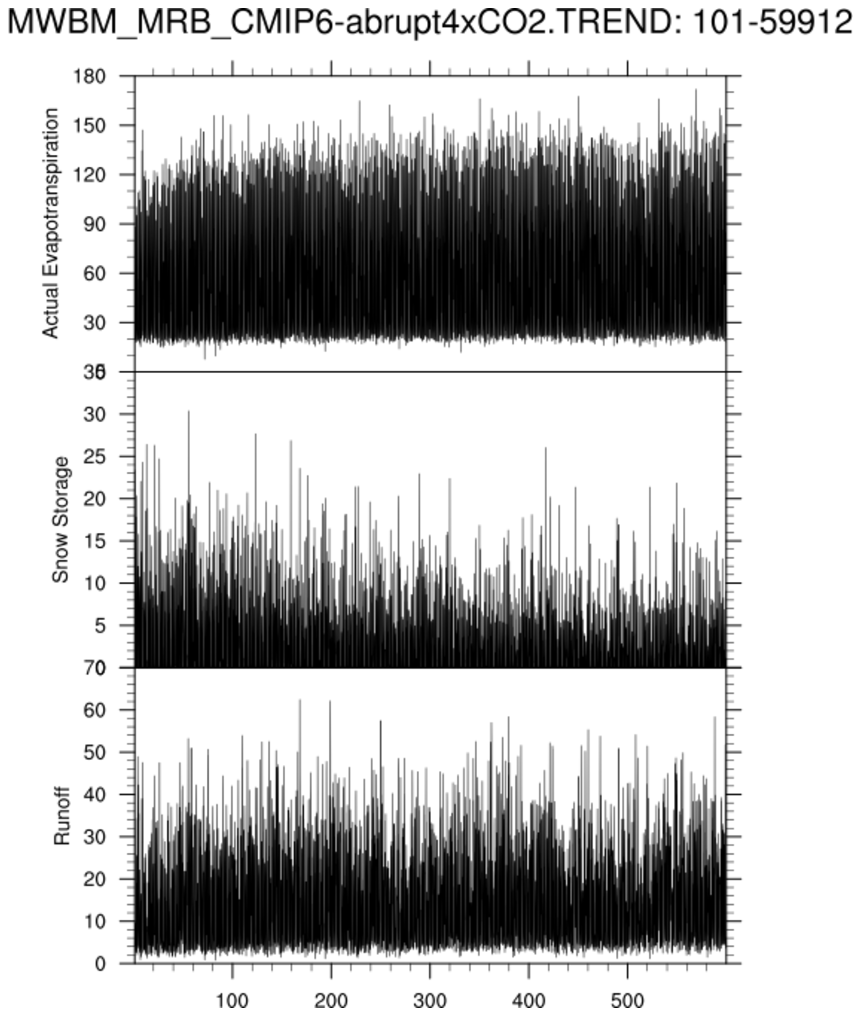
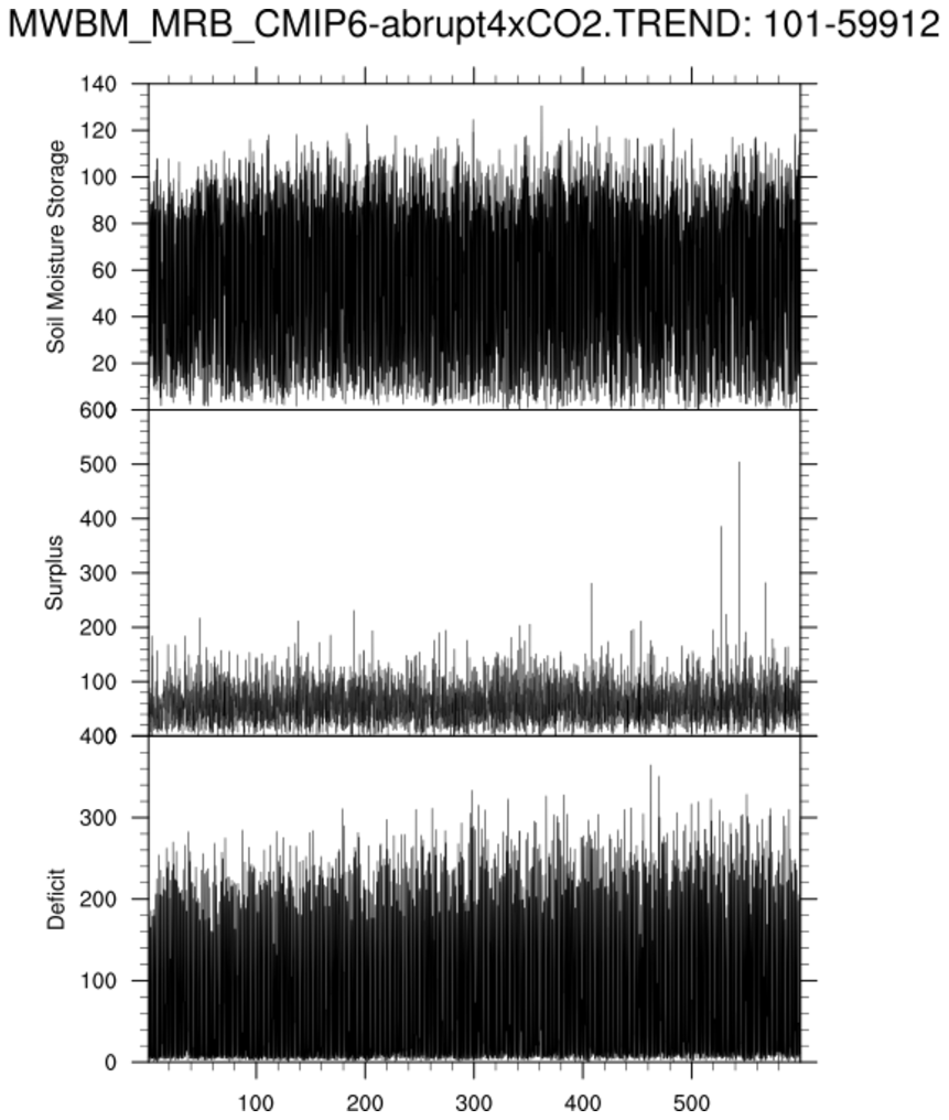
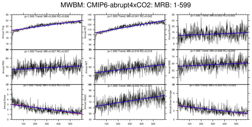
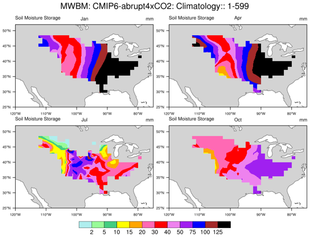
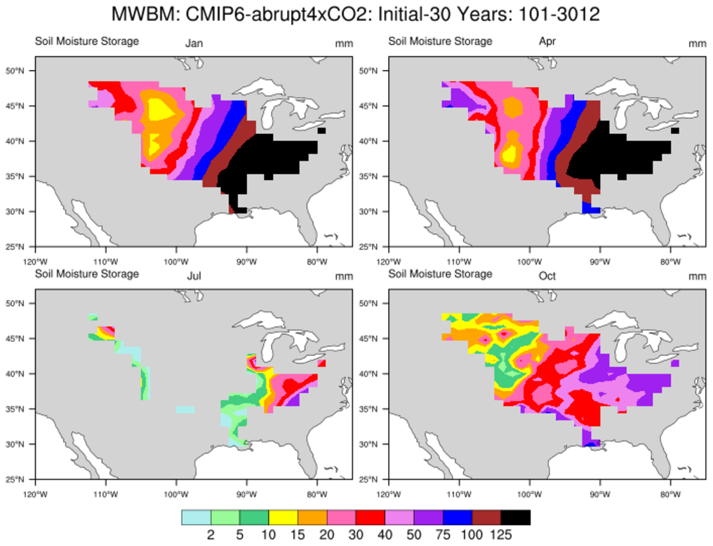
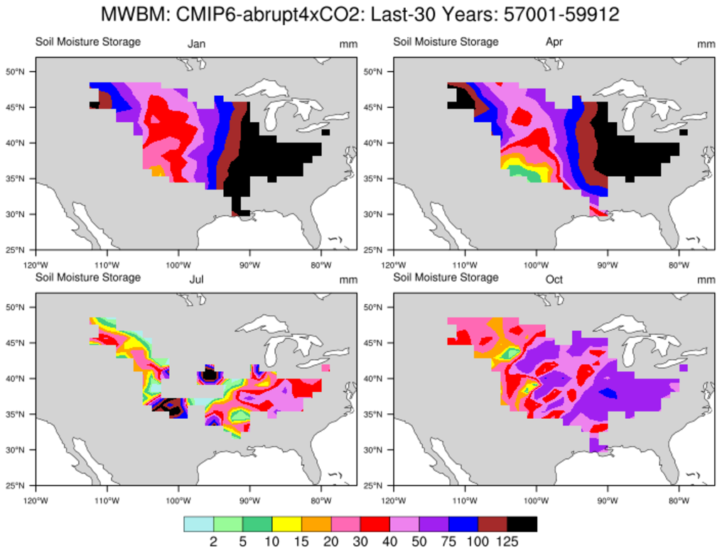
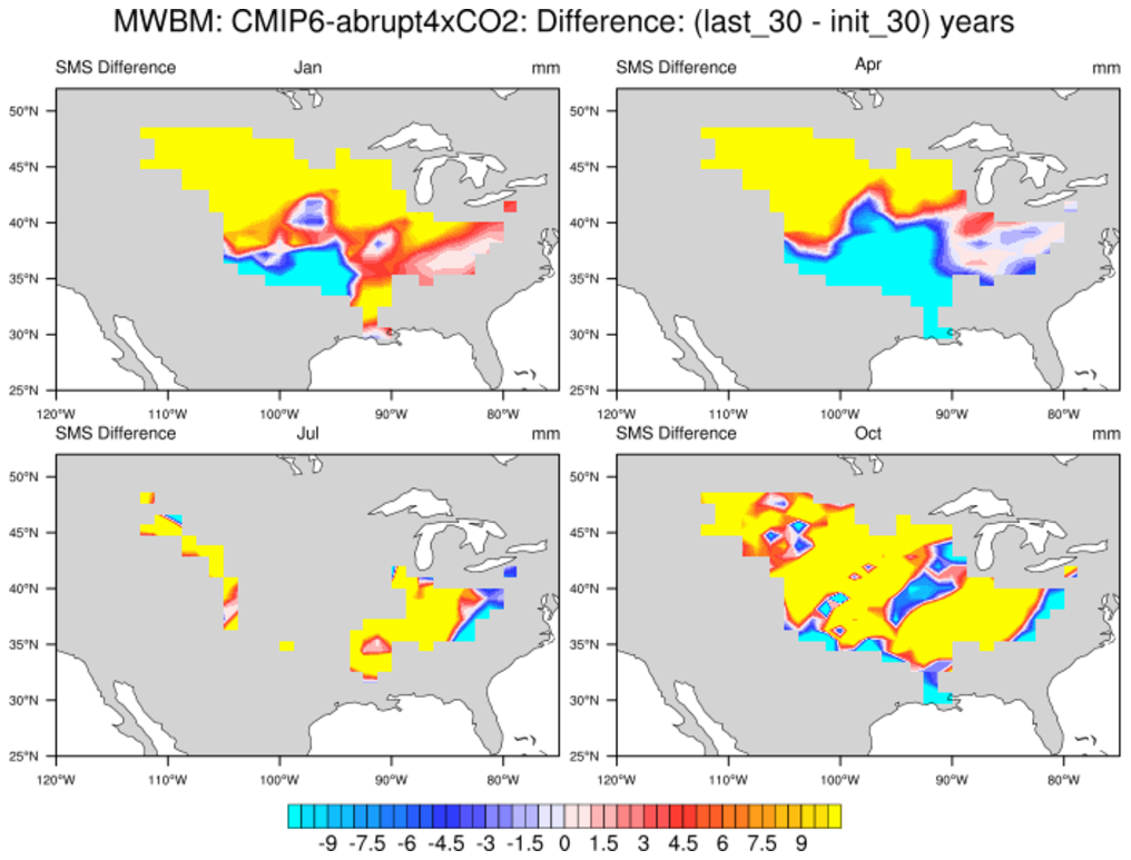
mwbm_5.ncl: Read CESM gridded (CMIP6-piControl) monthly data for 99 years. Extract data from a region which includes the Mississippi River Basin (MRB). Use a MRB shapefile [shapefile_4] to select grid points within the MRB. Print and plot time series of MRB's averaged hydrologic components. Calculate the trend of each source and derived component. Plot 30-year climatologies of soil moisture storage for the first and last 30-years. Plot the differences.
   + Figure 1: Initial input variables (Temperature, Precipitation, PET, Snow)
   + Figure 2: MWBM derived (a) Actual Evapotranspiration; (b) Snow Storage; (c) Runoff
   + Figure 3: MWBM derived (a) Soil Moisture Storage (SMS); (b) Surplus; (c) Deficit
   + Figure 4: Annual means with trend estimate: "p" greater/equal to 0.95 is significant
   + Figure 5: SMS: Monthly Climatology entire period
   + Figure 6: SMS: Monthly Climatology: First 30-years
   + Figure 7: SMS: Monthly Climatology: Last  30-years
   + Figure 8: SMS: Monthly Climatology Differences: (Last-First)-30 years
