The Gilleland et al reference below provides an overview of selected EV software.
NCL Home>
Application examples>
Data Analysis ||
Data files for some examples
 extval_1.ncl:
Plot the PDFs and CDFs of the
GEV distribution for user specified 'shape', 'scale' and 'center' parameters.
This example uses a function that returns to PDF and CDF
of the GEV distribution given the shape, center (location) and scale parameters:
extval_1.ncl:
Plot the PDFs and CDFs of the
GEV distribution for user specified 'shape', 'scale' and 'center' parameters.
This example uses a function that returns to PDF and CDF
of the GEV distribution given the shape, center (location) and scale parameters:
 extval_2.ncl:
Plot the PDFs and CDFs of the
Gumbel distribution
for user specified 'scale' and 'center' (location) parameters.
This example uses the following function:
extval_2.ncl:
Plot the PDFs and CDFs of the
Gumbel distribution
for user specified 'scale' and 'center' (location) parameters.
This example uses the following function:
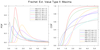 extval_3.ncl:
Plot the PDFs and CDFs of the Frechet distribution
for user specified 'shape', 'scale' and 'center' (location) parameters.
This example uses the following function:
extval_3.ncl:
Plot the PDFs and CDFs of the Frechet distribution
for user specified 'shape', 'scale' and 'center' (location) parameters.
This example uses the following function:
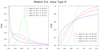 extval_4.ncl:
Plot the PDFs and CDFs of the
Weibull distribution
for user specified 'shape', 'scale' and 'center' (location) parameters.
This example uses the following function:
extval_4.ncl:
Plot the PDFs and CDFs of the
Weibull distribution
for user specified 'shape', 'scale' and 'center' (location) parameters.
This example uses the following function:
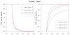
 extval_5.ncl:
Plot the PDFs and CDFs of the specified
Pareto distribution.
for user specified 'shape', 'scale' and 'center' (location) parameters.
Specifying ptype={0,1,2) creates the Pareto General, Type I and II distributions.
This example uses the following function:
extval_5.ncl:
Plot the PDFs and CDFs of the specified
Pareto distribution.
for user specified 'shape', 'scale' and 'center' (location) parameters.
Specifying ptype={0,1,2) creates the Pareto General, Type I and II distributions.
This example uses the following function:

 extval_6.ncl:
Example pages containing: tips | resources | functions/procedures
NCL: Basic Extreme Value Statistics
NCL has a small number of basic extreme value (EV) and recurrence statistical functions.
However, NCL is not R or S+ or Matlab or IDL or Excel
or Python's SciPy. These tools contain many more EV related functions.
That said: none of these tools is NCL either!
Extreme value theory (EVT) is a branch of statistics dealing with the extreme deviations from the median
of probability distributions. There exists a well elaborated statistical theory for extreme values.
It applies to (almost) all (univariate) extremal problems.
From EVT, extremes from a very large domain of stochastic processes
follow one of the three distribution types: Gumbel, Frechet/Pareto, or Weibull.
The generalized extreme value (GEV) distribution is a family of continuous probability distributions developed within EVT. The GEV combines three distributions into a single framework. The distributions are:
The GEV allows for a continuous range of possible shapes. The shape parameter, S, governs the tail behavior of the distribution. The sub-families defined by, S ~ 0, S > 0 and S < 0 correspond, respectively, to the Gumbel, Frechet and Weibull families. Note the differences in the ranges of interest for the three extreme value distributions: Gumbel is unlimited, Frechet has a lower limit, while the reversed Weibull has an upper limit.The GEV facilitates making decisions on which distribution is appropriate. The GEV distribution is often used as an approximation to model the minima or maxima of long (finite) sequences of random variables. In general, the GEV distribution provides better fit than the individual Gumbel, Frehet, and Weibull models. For example, in most hydrological applications, the distribution fitting is via the GEV as this avoids imposing the assumption that the distribution does not have a lower bound (as required by the Frechet distribution).
From Wikipedia:
The maximum value (or last order statistic) in a sample of a random variable following an exponential distribution approaches the Gumbel distribution closer with increasing sample size.[4] In hydrology, therefore, the Gumbel distribution is used to analyze such variables as monthly and annual maximum values of daily rainfall and river discharge volumes,[5] and also to describe droughts.
Most commonly, extreme value analyses focus on high extremes: maxima. It should be noted that dealing with minima follows the same approaches except for a sign reversal:
min[x(i)] = -max[-x(i)]
From Wikipedia:
Two approaches exist for practical extreme value analysis. The first method relies on deriving block maxima (minima) series as a preliminary step. In many situations it is customary and convenient to extract the annual maxima (minima), generating an "Annual Maxima Series" (AMS). The second method relies on extracting, from a continuous record, the peak values reached for any period during which values exceed a certain threshold (falls below a certain threshold). This method is generally referred to as the "Peak Over Threshold" [1] method (POT) and can lead to several or no values being extracted in any given year
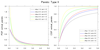
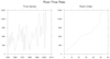
Example 6 (below) offers a sample block maxima approach based on extracting the maximum rate of river flow ineach year.
An estimate of the likelihood of an event, such as a flood or heat wave, is commonly called the
return period.
However, other terms are used, including:
repeat interval, recurrence interval, exceedance probability,
expected frequency and return interval. These terms are synonymous.
General References:
   Alexandersson, H. et al (2001): Extreme Value Analysis in Nordic countries:
                                   Pilot Studies of minimum temperatue and maximum daily precipitation
                                   and a review of methods in use

   Coles, S. (2001): An Introduction to Statistical Modeling of Extreme Values.
   Springer ISBN 978-1-4471-3675-0

   Coles, S. and A. Davison (2008):  Statistical Modelling of Extreme Values

   Gilleland, E. et al (2013): A software review for extreme value analysis
   Extremes 16:103-119
   DOI 10.1007/s10687-012-0155-0

   Gilleland, E. and Katz, R.W. (2014): extRemes 2.0:  An Extreme Value Analysis Package R

   Gong, S. (2012): Estimation of hot and cold spells with extreme value theory.
   U.U.D.M. Project Report 2012:19 (Uppsala Universitet).

   Katz, R. (???): Introduction to Statistical Theory of Extreme Values

   Katz, R. et al (2002):
Statistics of Extremes in Hydrology. Advances in Water Resources: 25: 1287–1304.

   NASA: Generalized Extreme Value Distribution and Calculation of Return Value

   Rieder, H.E. (2014):  Extreme Value Theory: A primer.
   Lamont Doherty Earth Observatory.


   Wikipedia: (a) Extreme Value Theory
              (b) Generalized Extreme Value Distribution

   Wilks, D. (2006): Statistical Methods in the Atmospheric Sciences. Academic Press.
NCL (6.4/5.0) currently has several GEV statistical functions.
Currently, the only ones documented are:
- extval_mlegev
- extval_mlegam
- extval_mlegev
- extval_gev
- extval_gumbel
- extval_frechet
- extval_pareto
- extval_weibull
- extval_recurrence_table
- extval_return_period
- extval_return_prob
- others may be added
- shape - affects the distribution shape [ ;-) ]
- scale - stretches or shrinks the distribution
- center, location - shifts the distribution
The extval_mlegev and extval_mlegam provide maximum-liklihood estimates of these parameters for the GEV and Gamma distributions, respectively. The method of moments can readily be used to derive parameter estimates for other extreme value distributions. However, the moment method ahs some issues (biases).
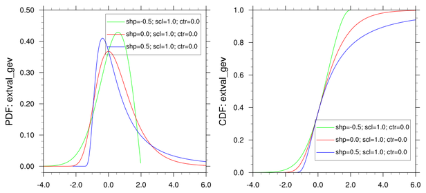
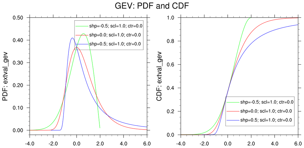 extval_1.ncl:
Plot the PDFs and CDFs of the
GEV distribution for user specified 'shape', 'scale' and 'center' parameters.
This example uses a function that returns to PDF and CDF
of the GEV distribution given the shape, center (location) and scale parameters:
extval_1.ncl:
Plot the PDFs and CDFs of the
GEV distribution for user specified 'shape', 'scale' and 'center' parameters.
This example uses a function that returns to PDF and CDF
of the GEV distribution given the shape, center (location) and scale parameters:
pdfcdf = extval_gev(x, shape, scale, center, 0) ; [/ PDF, CDF /]
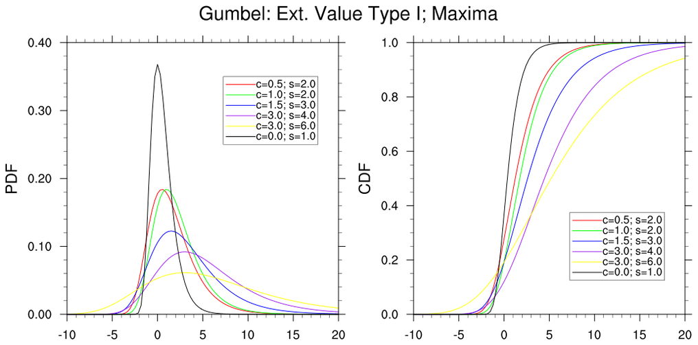
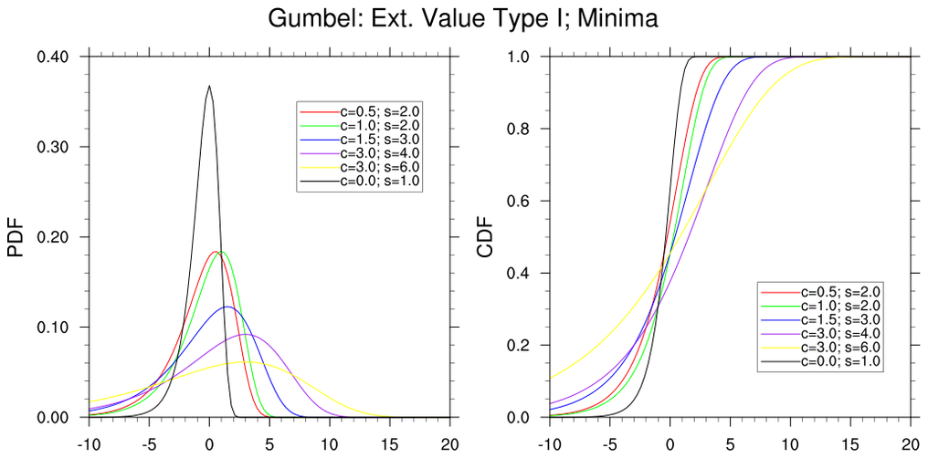 extval_2.ncl:
Plot the PDFs and CDFs of the
Gumbel distribution
for user specified 'scale' and 'center' (location) parameters.
This example uses the following function:
extval_2.ncl:
Plot the PDFs and CDFs of the
Gumbel distribution
for user specified 'scale' and 'center' (location) parameters.
This example uses the following function:
pdfcdf = extval_gumbel(x, scale, center, 0) ; [/ PDF, CDF /]
Note: The extreme value Type I distribution has two forms.
One is based on the smallest extreme ('minima') and the other
is based on the largest extreme ('maxima').
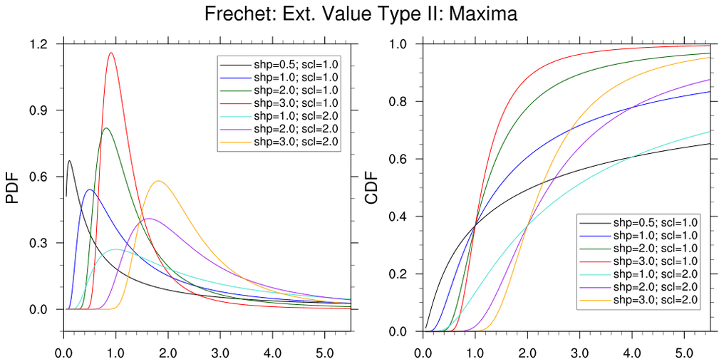 extval_3.ncl:
Plot the PDFs and CDFs of the Frechet distribution
for user specified 'shape', 'scale' and 'center' (location) parameters.
This example uses the following function:
extval_3.ncl:
Plot the PDFs and CDFs of the Frechet distribution
for user specified 'shape', 'scale' and 'center' (location) parameters.
This example uses the following function:
pdfcdf = extval_frechet(x, shape, scale, center, 0) ; [/ PDF, CDF /]
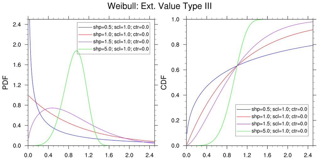 extval_4.ncl:
Plot the PDFs and CDFs of the
Weibull distribution
for user specified 'shape', 'scale' and 'center' (location) parameters.
This example uses the following function:
extval_4.ncl:
Plot the PDFs and CDFs of the
Weibull distribution
for user specified 'shape', 'scale' and 'center' (location) parameters.
This example uses the following function:
pdfcdf = extval_weibull(x, shape, scale, center, 0) ; [/ PDF, CDF /]
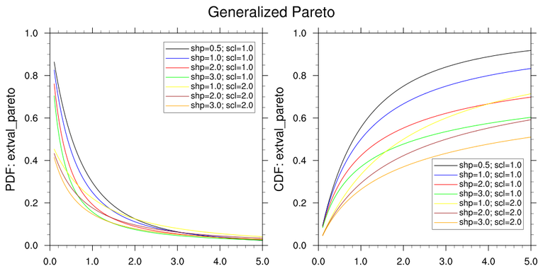
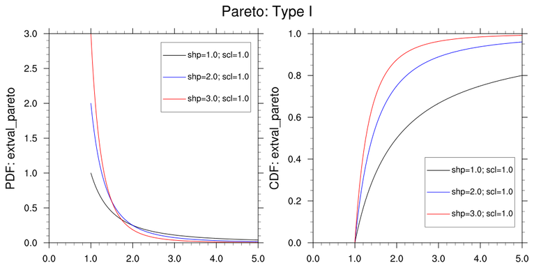
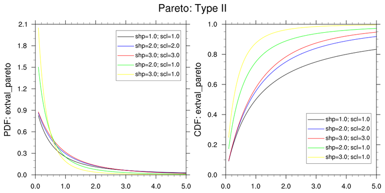 extval_5.ncl:
Plot the PDFs and CDFs of the specified
Pareto distribution.
for user specified 'shape', 'scale' and 'center' (location) parameters.
Specifying ptype={0,1,2) creates the Pareto General, Type I and II distributions.
This example uses the following function:
extval_5.ncl:
Plot the PDFs and CDFs of the specified
Pareto distribution.
for user specified 'shape', 'scale' and 'center' (location) parameters.
Specifying ptype={0,1,2) creates the Pareto General, Type I and II distributions.
This example uses the following function:
pdfcdf = extval_pareto(x, shape, scale, center, ptype, 0) ; [/ PDF, CDF /]
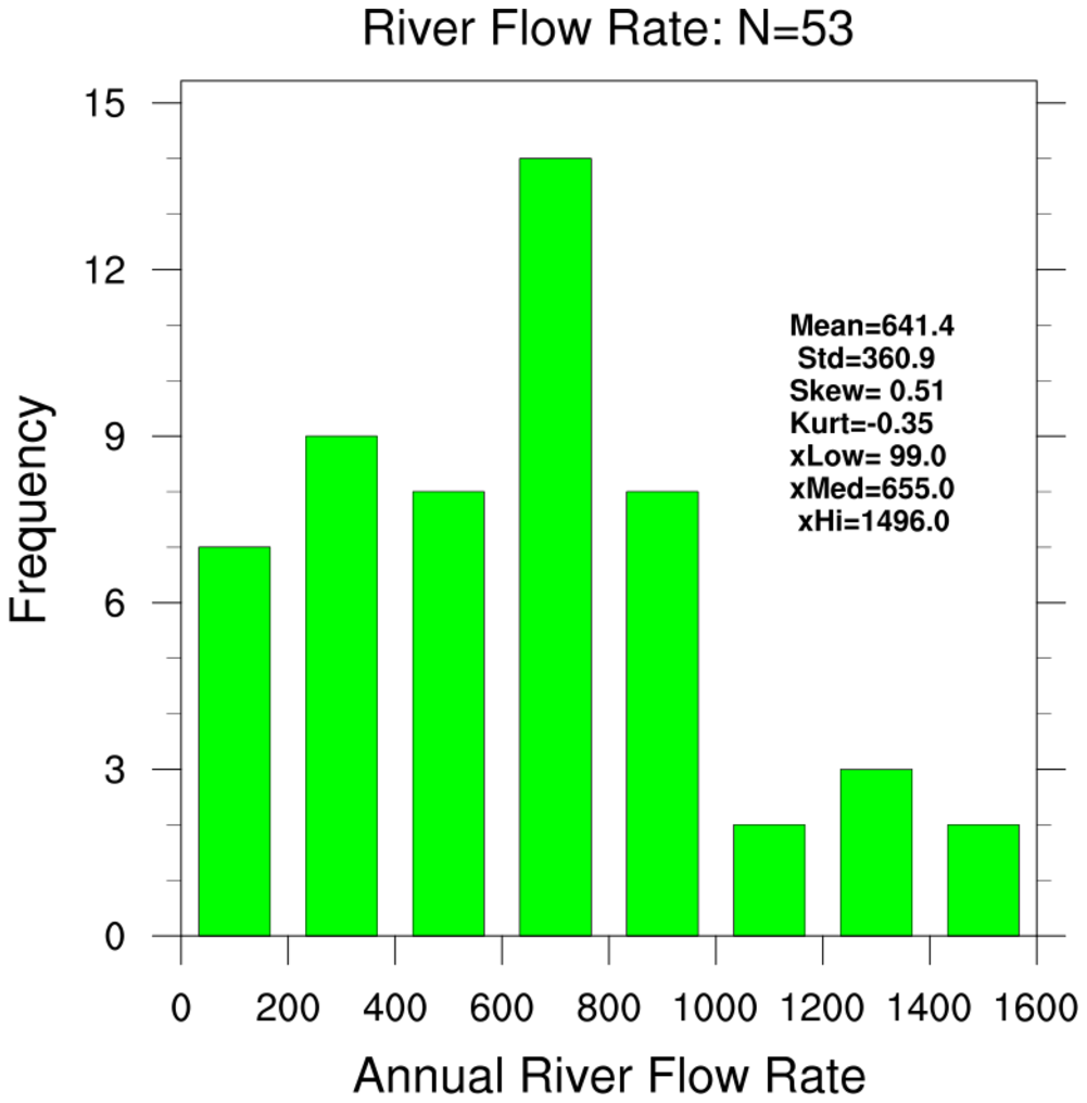
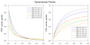
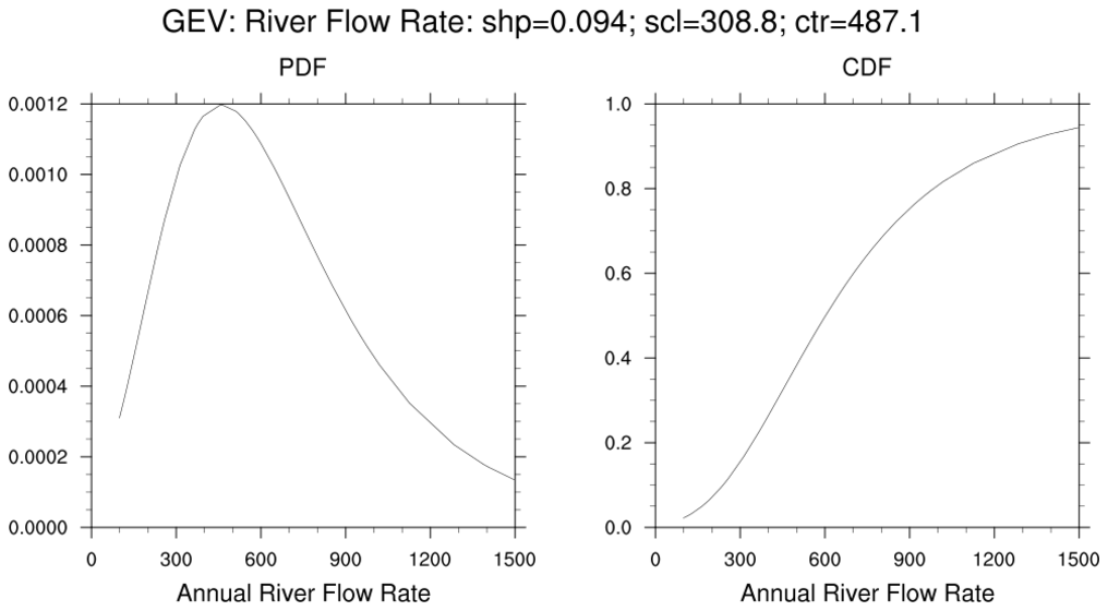 extval_6.ncl:
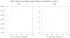
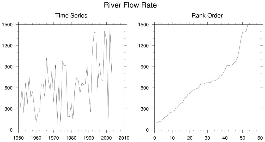
Examine 'Maximum Annual River Flow Rate' data using graphics and conventional statistics. Derive the shape, scale and center (location) parameters using the extval_mlegev function. Using the returned parameter estimates calculate the PDF and CDF associated with the GEV distribution using the extval_gev function.
The shape parameter is near zero (S=0.094). Hence, the distribuion is similar to the Gumbel distribution.
This example can be viewed as a 'block maxima' approach. Here the maximum river flow rate is recorded for each year. This selected subset of maximum flow rates was used for the statistics.
Example 5 for the extval_recurrence_table uses the the same data. It provides a 'table-based' approach to examining the data.