      (dZ/dlon) is the zonal gradient
      (dZ/dlat) is the meridional gradient
NCL Home>
Application examples>
Data sets ||
Data files for some examples
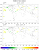
 gradient_1.ncl:
Using a global gaussian rectilinear grid, calculate the meridional and zonal gradients
using two independent methods. The first uses the "highly accurate"
spherical harmonic procedure gradsg. The second method uses
simple centered finite differences
(grad_latlon_cfd).
gradient_1.ncl:
Using a global gaussian rectilinear grid, calculate the meridional and zonal gradients
using two independent methods. The first uses the "highly accurate"
spherical harmonic procedure gradsg. The second method uses
simple centered finite differences
(grad_latlon_cfd).
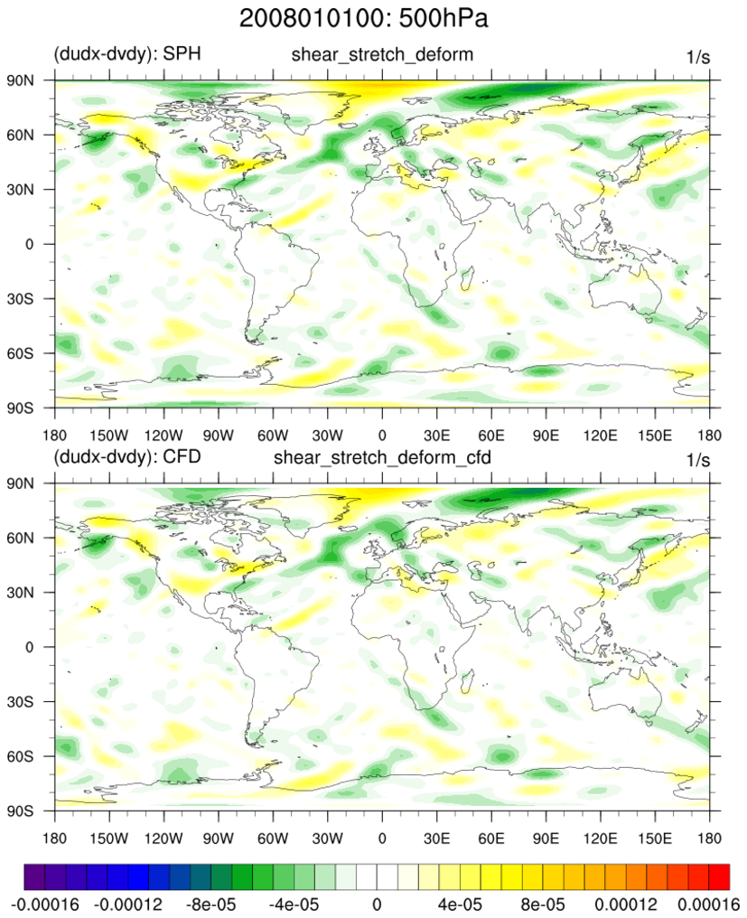
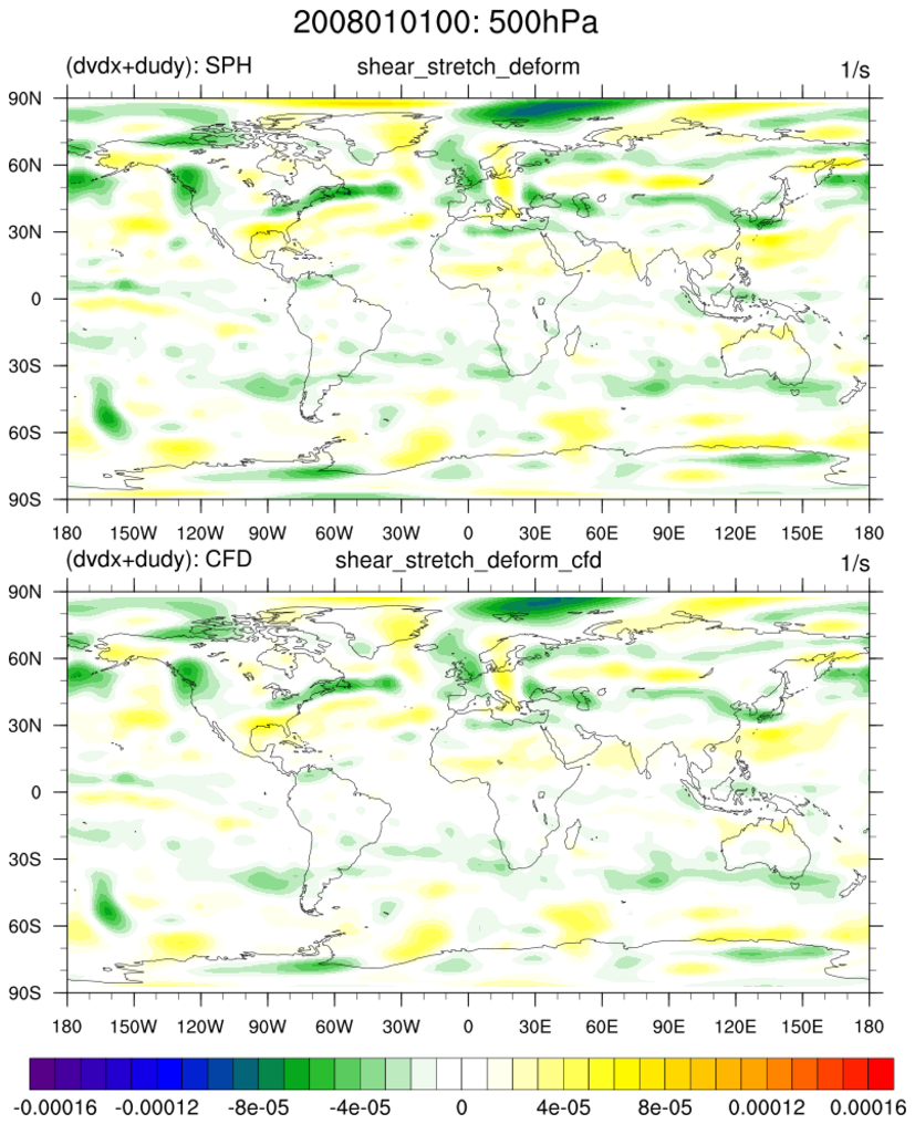
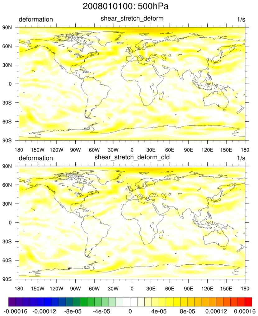
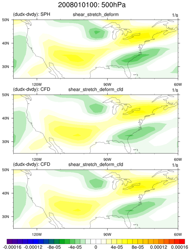
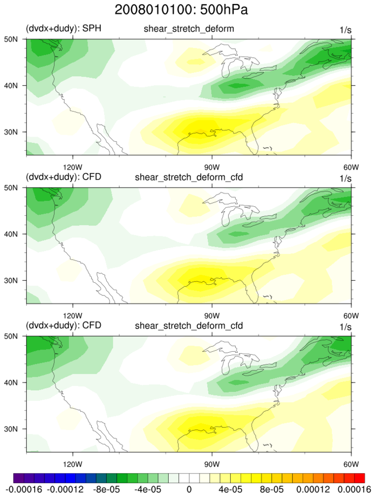
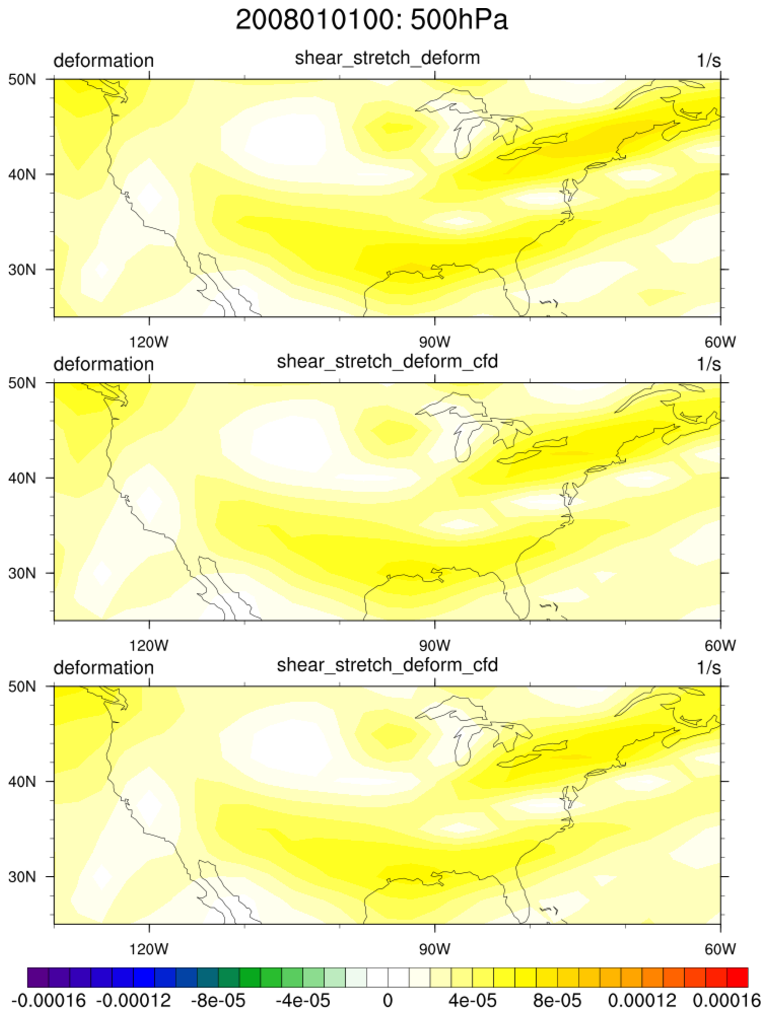
 shear_stretch_deform_1.ncl:
Using a global rectilinear grid, calculate the shear, stretch and deformation.
The first method uses the "highly accurate" spherical harmonic procedure:
(shear_stretch_deform).
The second method uses centered finite differences:
(shear_stretch_deform_cfd).
shear_stretch_deform_1.ncl:
Using a global rectilinear grid, calculate the shear, stretch and deformation.
The first method uses the "highly accurate" spherical harmonic procedure:
(shear_stretch_deform).
The second method uses centered finite differences:
(shear_stretch_deform_cfd).
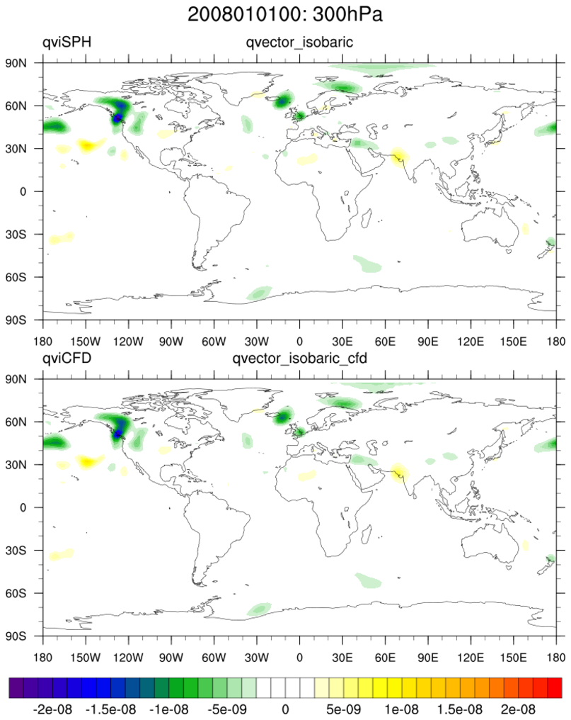
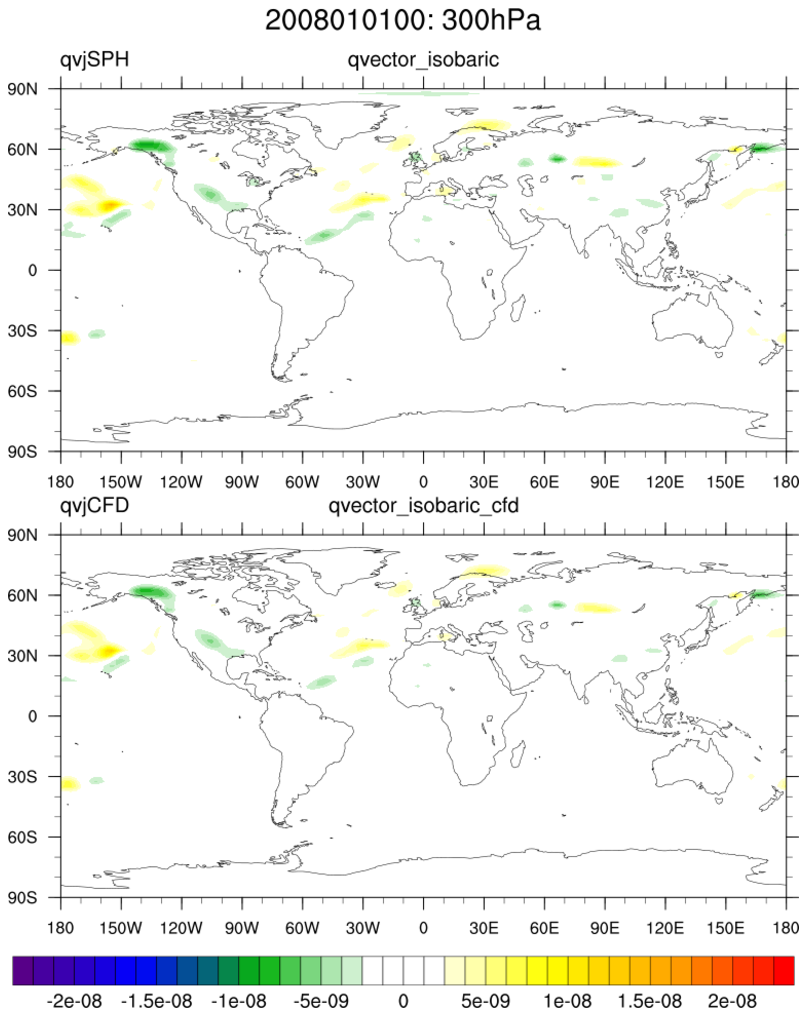
 qvector_1.ncl:
Using a global rectilinear grid, calculate the Q-vector information..
The first method uses the "highly accurate" spherical harmonic procedure:
(qvector_isobaric).
The second method uses centered finite differences:
(qvector_isobaric_cfd).
qvector_1.ncl:
Using a global rectilinear grid, calculate the Q-vector information..
The first method uses the "highly accurate" spherical harmonic procedure:
(qvector_isobaric).
The second method uses centered finite differences:
(qvector_isobaric_cfd).
Example pages containing:
tips |
resources |
functions/procedures
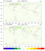
Meridional and Zonal gradients
The gradient is a physical quantity that describes the rate at which a quantity
changes. Meridional and zonal gradients represent rates of change in the
meridional (latitudinal) and zonal (longitudinal) directions.
Mathematically, these quantities are obtained by applying the del operator to
a variable which is a function of position. Specifically, for variable Z

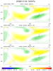
 gradient_1.ncl:
Using a global gaussian rectilinear grid, calculate the meridional and zonal gradients
using two independent methods. The first uses the "highly accurate"
spherical harmonic procedure gradsg. The second method uses
simple centered finite differences
(grad_latlon_cfd).
gradient_1.ncl:
Using a global gaussian rectilinear grid, calculate the meridional and zonal gradients
using two independent methods. The first uses the "highly accurate"
spherical harmonic procedure gradsg. The second method uses
simple centered finite differences
(grad_latlon_cfd).
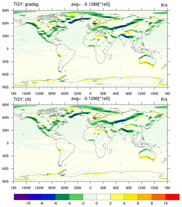
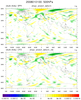
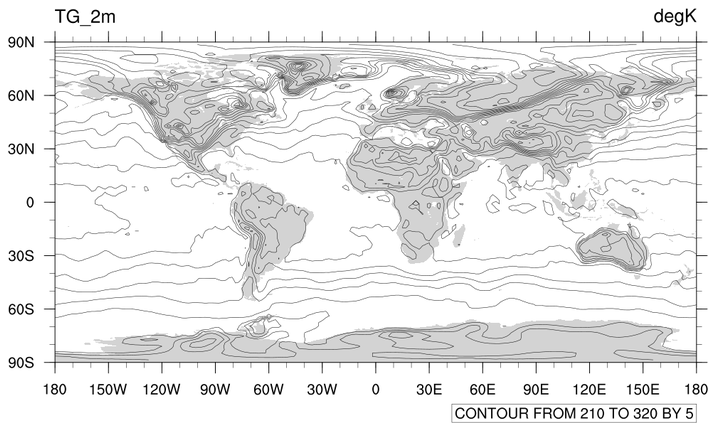
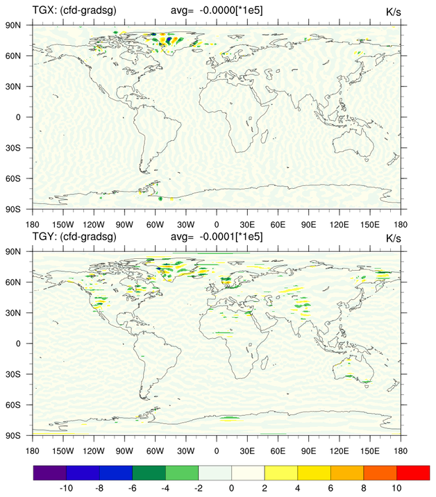
The 2-meter temperature variable was used because it has tight gradients and can be a bit noisy. These characteristics will amplify the differences beween the two approaches. If (say) a 500 hPa variable had been chosen the differences would be smaller.
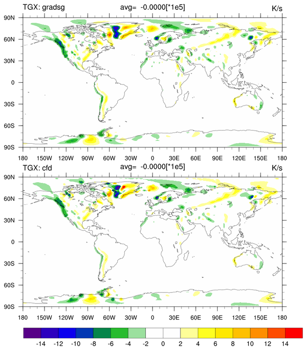
Differences between the two approaches are explained because the centered finite differences are less accurate. For example, the 2nd plot on the left displays the meridional gradients derived from using the gradsg procedure (top; labeled 'TGY: grads') and the grad_latlon_cfd function (bottom; labeled 'TGY: cfd'). The visual results from gradsg show more detail as seen by the deeper colors. The grad_latlon_cfd are smoother and lack the small scale detail. (Of course, if the small scale detail are the result of noise, do you want them?) The rightmost plot displays the actual numerical differences of the TGX (top) and TGY (bottom) gradients.
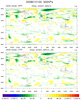
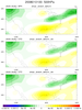
 shear_stretch_deform_1.ncl:
Using a global rectilinear grid, calculate the shear, stretch and deformation.
The first method uses the "highly accurate" spherical harmonic procedure:
(shear_stretch_deform).
The second method uses centered finite differences:
(shear_stretch_deform_cfd).
shear_stretch_deform_1.ncl:
Using a global rectilinear grid, calculate the shear, stretch and deformation.
The first method uses the "highly accurate" spherical harmonic procedure:
(shear_stretch_deform).
The second method uses centered finite differences:
(shear_stretch_deform_cfd).
The source variables are on a global 2.5 degree grid and are relatively smooth. Hence, there are little differences between the two methods.
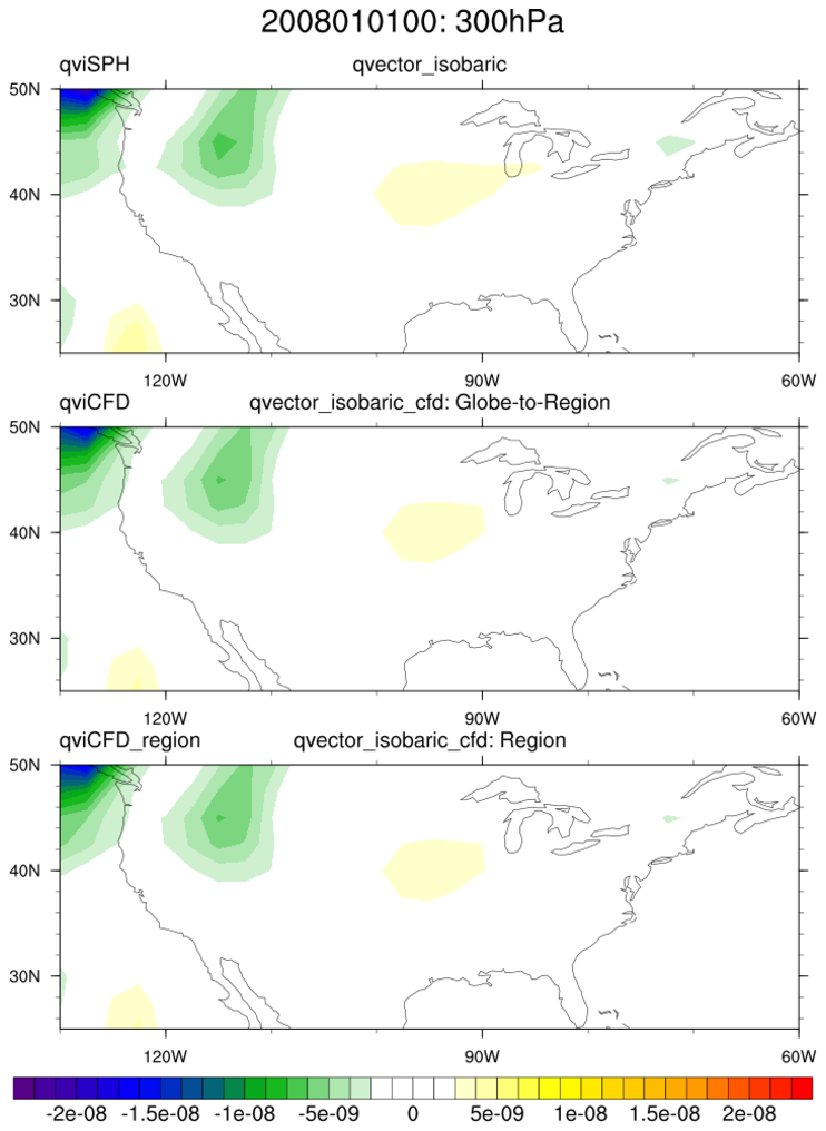
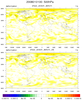
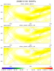
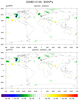
 qvector_1.ncl:
Using a global rectilinear grid, calculate the Q-vector information..
The first method uses the "highly accurate" spherical harmonic procedure:
(qvector_isobaric).
The second method uses centered finite differences:
(qvector_isobaric_cfd).
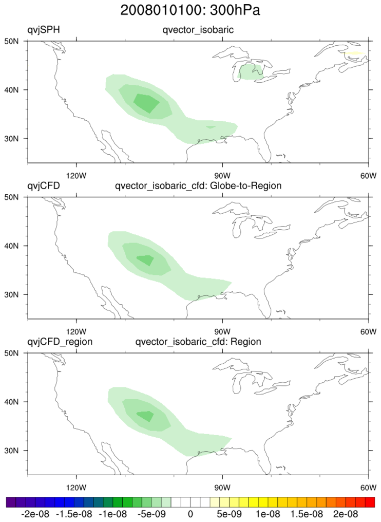
qvector_1.ncl:
Using a global rectilinear grid, calculate the Q-vector information..
The first method uses the "highly accurate" spherical harmonic procedure:
(qvector_isobaric).
The second method uses centered finite differences:
(qvector_isobaric_cfd).
The source variables are on a global 2.5 degree grid and are relatively smooth. Hence, there are little differences between the two methods.