NCL: Atmospheric and Oceanographic Indices

A climate index is a simple diagnostic quantity that is used to characterize an aspect of a geophysical system such as a circulation pattern. A variety of methods have been used to derive assorted indices. Classically, selected station or grid point data have been used (eg., Southern Oscillation Index, Niño 3.4). Other indices are based upon empirical orthogonal functions (EOFs; eg., Artic Oscillation) or a Rotated EOF (REOF; eg, Pacific-North American). Most indices use a single variable (eg., sea level pressure) while others, such as the Palmer Drought Index (PDI) use a combination of variables (eg, temperature and precipitation). Unfortunately, some indices are similarly named which results in user confusion. Further, use of different source data sets, different base periods and, where applicable, different normalizations can yield different index values.

Monthly values can be noisy so the are often smoothed via a unweighted (runave_n, runave_n_Wrap) or weighted running average (wgt_runave_n, wgt_runave_n_Wrap). For the latter, the filwgts_lanczos function may be used to create a set of weights that have characteristics specified by the user.

Note that calculated index values may differ from those at various web sites. Commonly, the reason is that different data sets were used. Each dataset was created via different methodologies and source datasets. It is unlikely that the derived indices will differ in any substantive way.

The Climate Data Guide provides links and descriptions to selected climate indices.

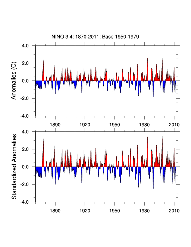
indices_nino_1.ncl: Read sea surface temperatures for a selected region and time period from a netCDF file. Compute a climatology for a specified base period; create anomalies from the base climatology ; average all the anoamlies to create an area averaged time series; create a standardized time series by dividing the raw anomalies by the period standard deviation.

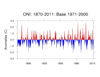
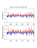
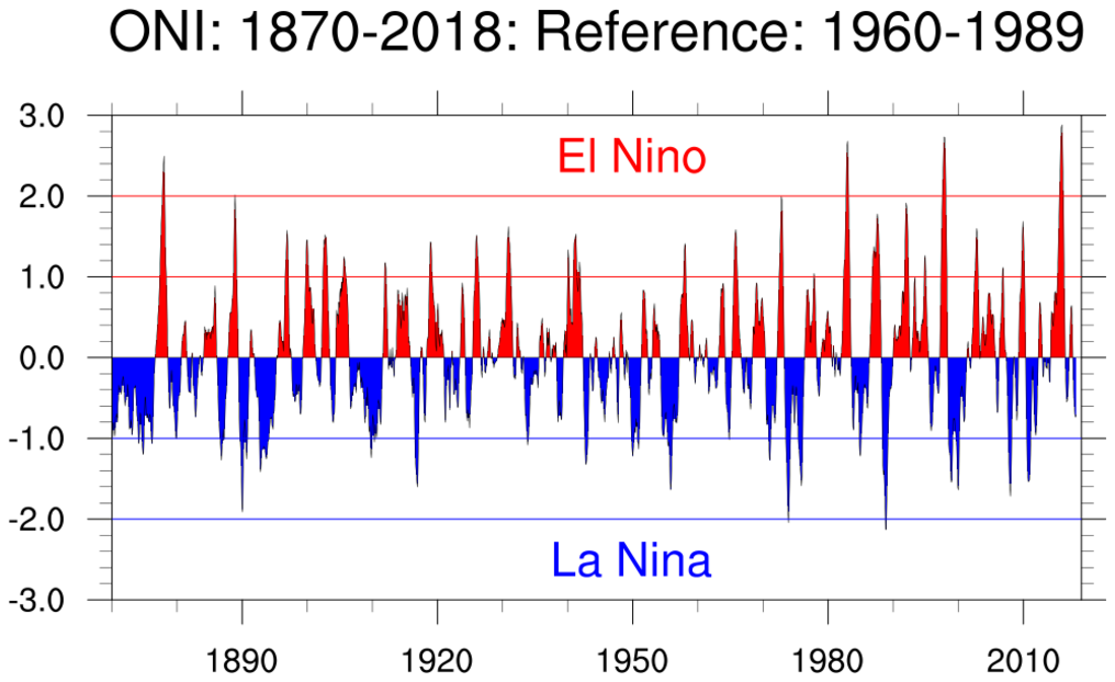
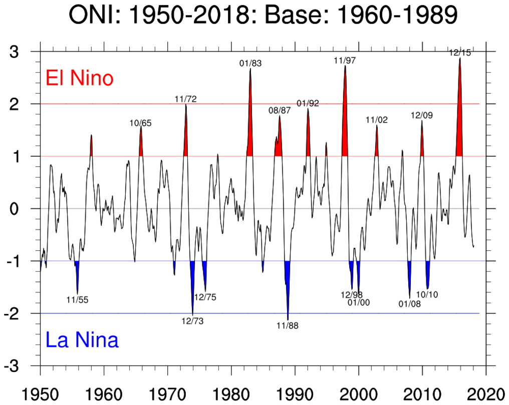
indices_oni_1.ncl: NOAA's operational definitions of El Niño and La Niña conditions are based upon the Oceanic Niño Index [ONI]. The ONI is defined as the 3-month running means of SST anomalies in the Niño 3.4 region [5N-5S, 120-170W]. The anomalies are derived from the 1971-2000 SST climatology.

The Niño 3.4 anomalies may be thought of as representing the average equatorial SSTs across the Pacific from about the dateline to the South American coast. To be classified as a full-fledged El Niño and La Niña episode the ONI must exceed +0.5 [El Niño] or -0.5 [La Niña] for at least five consecutive months.

indices_oni_2.ncl: This is a variation of the previous ONI example. Text and reference lines are added. The 'strong' El Niño and La Niña are marked on the time series. The table spans 1950 onward.

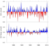
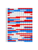
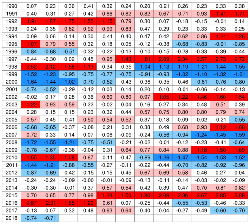
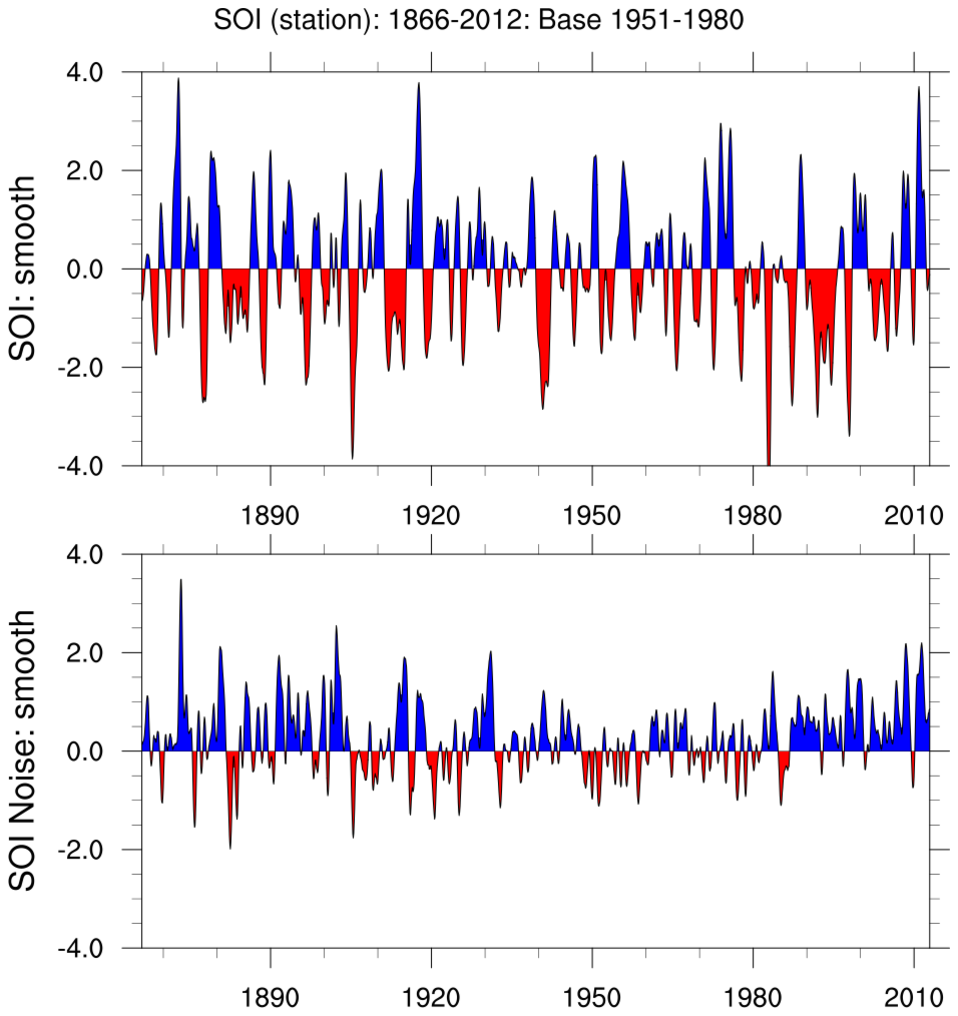
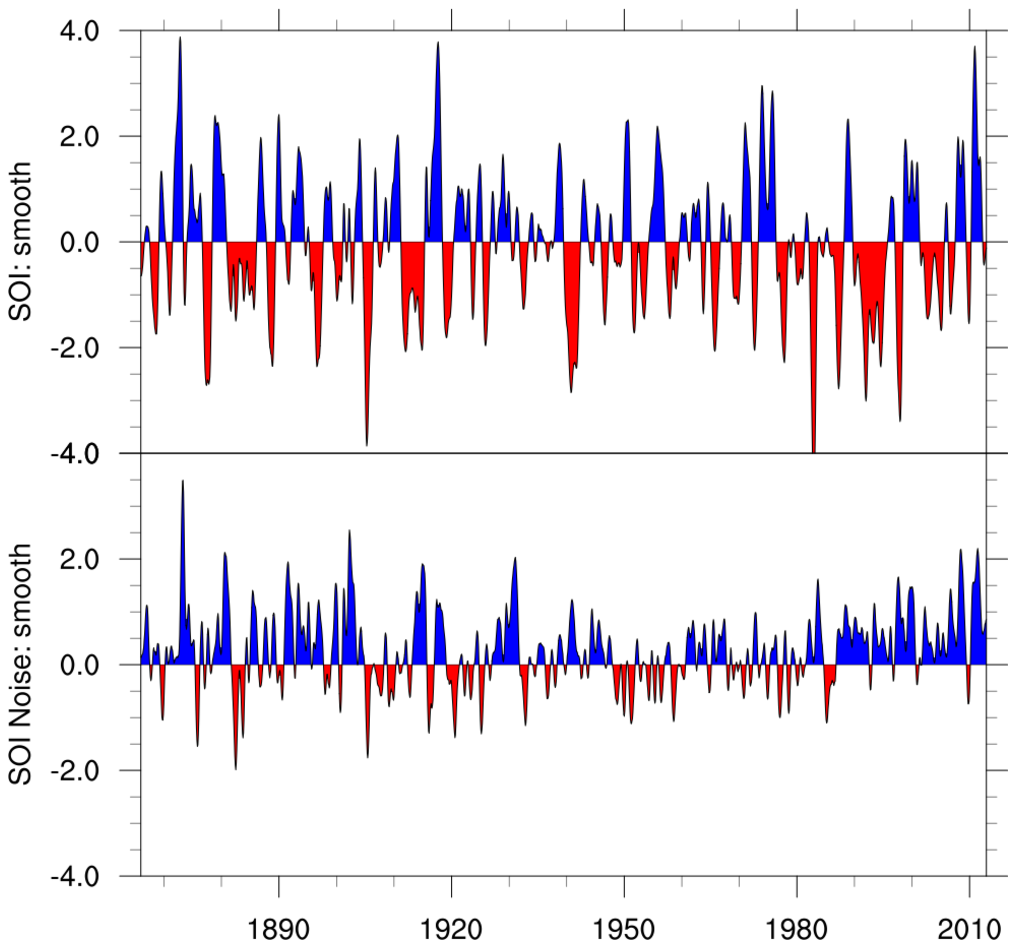
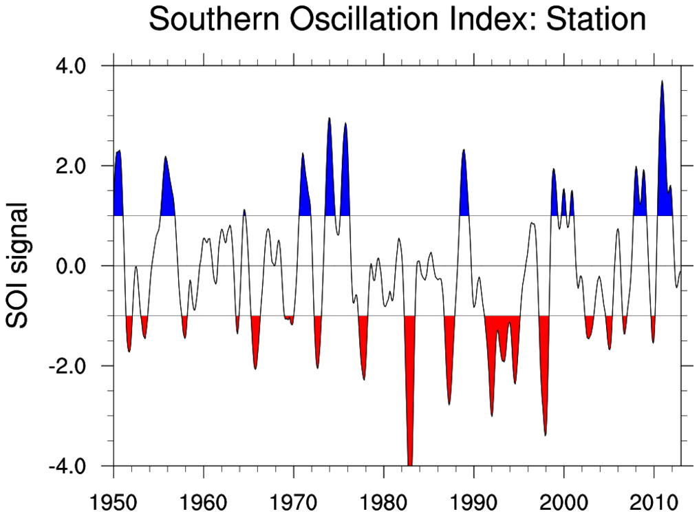
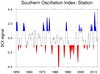indices_soi_1.ncl: Read ascii (text) files containing station sea level pressures from Tahiti and Darwin. Compute the Southern Oscillation Index (SOI) signal and noise values. Make 3 plots for illustration: (a) a standard panel plot; (b) the plots 'attached'; and, (c) a plot showing all SOI greater than plus/minus one standard deviation.

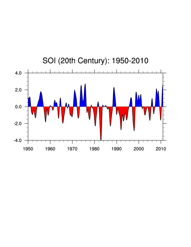
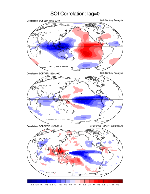
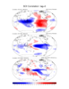indices_soi_2.ncl: Read gridded sea level pressure from the 20th Century Reanalysis; use proxy grid points near Tahiti and Darwin to construct an SOI time series spanning 1950-2010; perform lag-0 correlations between the SOI and SLP; SOI and temperature; and, SOI and preciptation. The later uses the GPCP data which spans 1979-2010. To more clearly delineate the main pattern structure correlations between, -0.1 and +0.1 were set to _FillValue.

FYI: The linear correlation between the station based SOI (previous example) and the SOI derived from the 20th Century Reanalysis for the 1950-2010 period is 0.96.

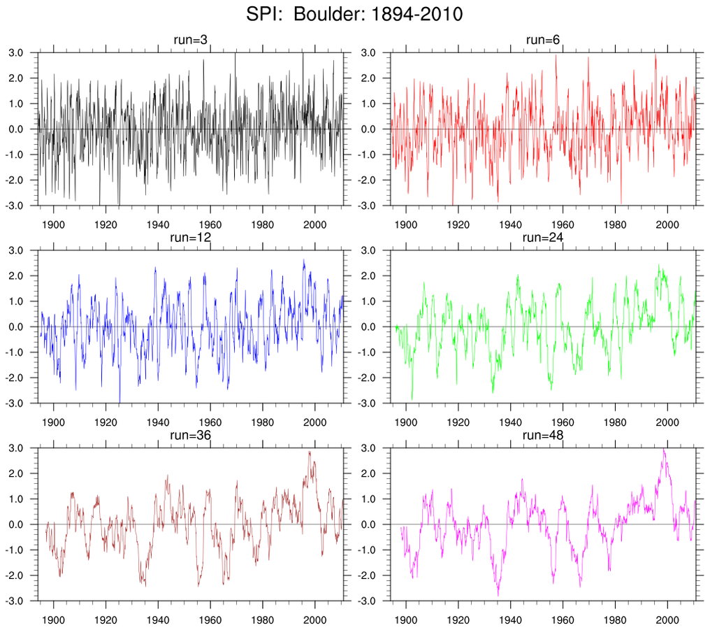
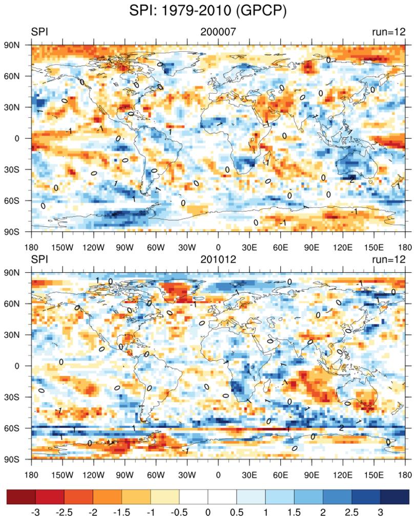
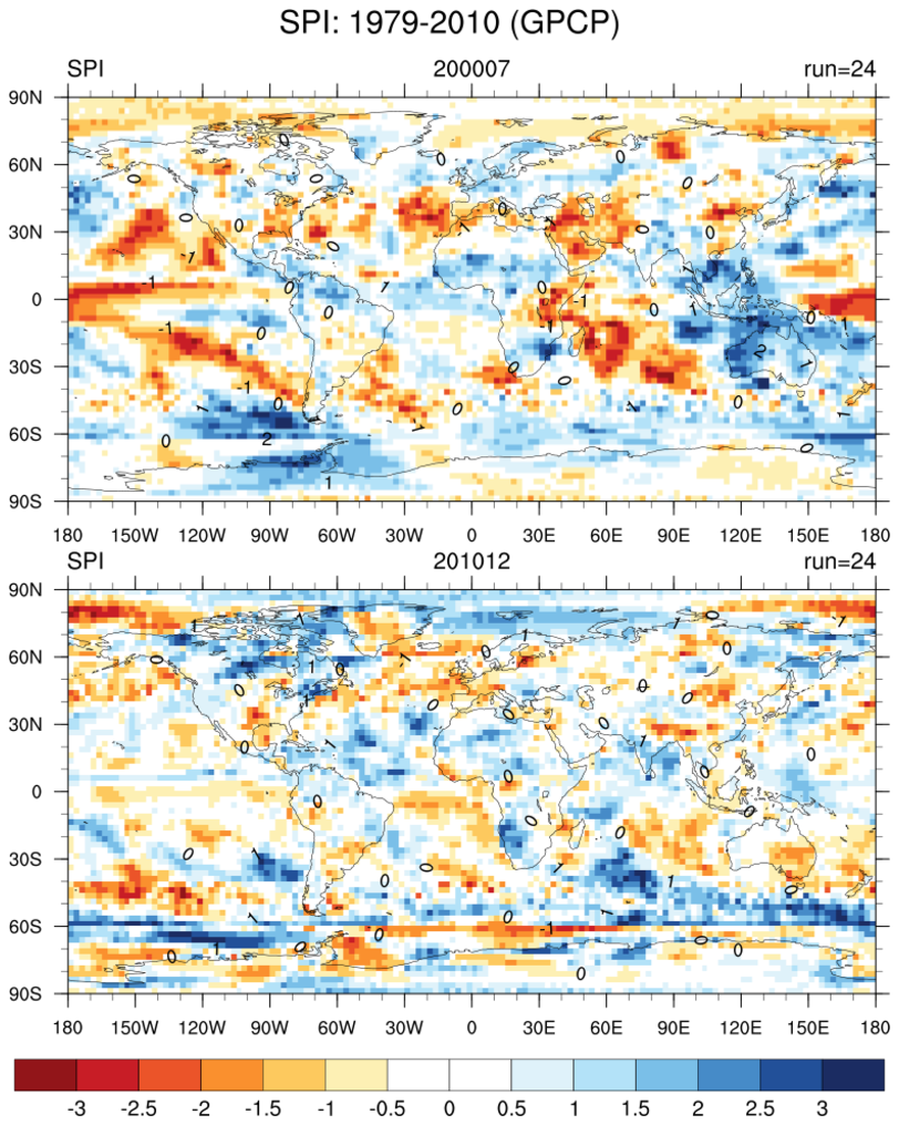
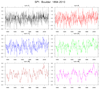spi_1.ncl: Read Boulder, CO monthly precipitation and compute the SPI for different run lengths. Plot the time series.

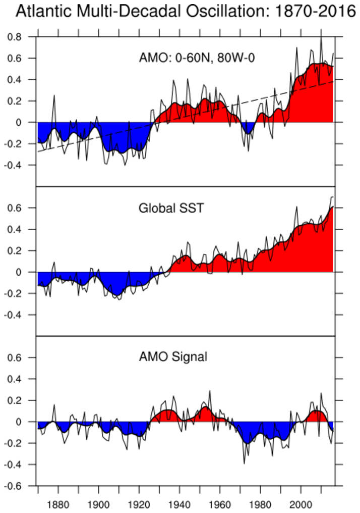
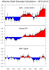spi_2.ncl: Read the monthly Global Precipitation Climatology Project (GPCP) spanning 1979-2010 and compute the SPI for 12 and 24 month run lengths. Plot two arbitrarily selected maps.

index_amo_1.ncl: Create the Atlantic Multi-decadal Oscillation (AMO) index (signal). Optionally, output a netCDF file and/or simple ascii files and a with assorted time series.

With appropriate script changes, any SST data set can be used. This example uses the Hurrell et al (2008). The file containing the SST data may be downloaded from:


    ftp ftp.cgd.ucar.edu
    anonymous
    email
    cd archive/SSTICE
    prompt 
    ls
    get MODEL.SST.HAD187001-198110.OI198111-201703.nc.gz
    quit

The 'gzip -d ' command must be used prior to use (gzip'd file size is > 270MB ]. The file is updated once per year. Hence, the last 'yyyy03' may change.