NCL: NLOM model (subregions)

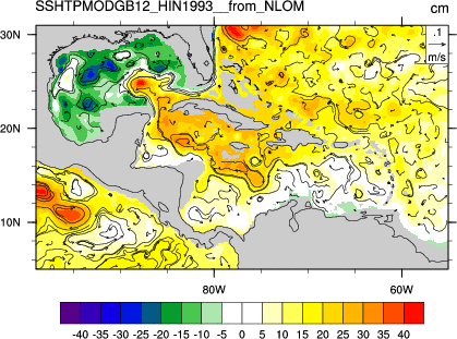
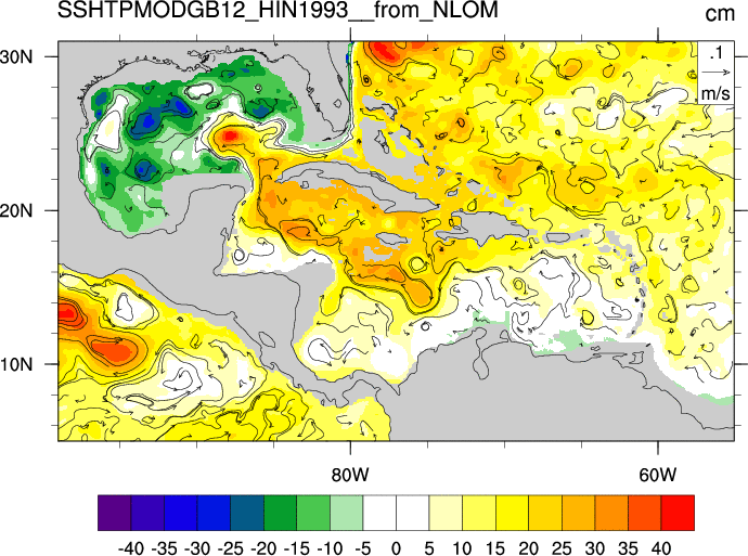nlom_1.ncl: Creates single pane images of scalar variables overlaid by vectors.

gsn_csm_vector_scalar_map_ce is the plot interface that puts plots vectors on top a scalar field.

NLOM lat/lon coordinate variables are missing an attribute that the plot interfaces look for. The result is a warning message. This can be eliminated by assigning the attributes:

  ssh&Longitude@units = "degrees_east"
  ssh&Latitude@units  = "degrees_north"

Options to the gsn_csm plot templates are controlled by resources. In this script: cnFillOn = True turns on the color while cnFillMode="RasterFill" turns on raster color. NLOM data file are quite large, and a raster plot will be created faster than a colorfill plot. cnLinesOn = False, turns off the contour lines which must be done when rasterizing.

cnMissingValFillColor sets the color of any missing values within the data. In this case the color was set to match the default gray continents.

There are three coastline databases in NCL.
There are numerous things to do with vectors.

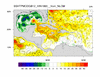
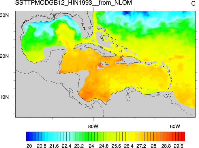nlom_2.ncl: Plots a scalar field and masks out the pacific with a fortran subroutine.

Use WRAPIT to compile mask.f. Note that WRAPIT comes with the NCL binaries.

gsn_csm_contour_map_ce is the plot interface that puts contour data onto a cylindrical equidistant projection.

gsnMaximize will enlarge and rotate a plot to maximize its size on a page.

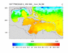
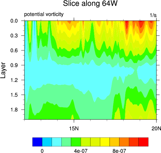nlom_3.ncl: A slice plot along a specified longitude.

Eventually we will have to run the vertical array through an interpolator.

NLOM data is separated out by layer into different files. In order to create a slice plot that spans multiple files, we need to combine these together. This is done via a loop. This process unfortunately means that there is no meta data associated with the new, concatenated variable. These must be assigned.

The "!" operator is used to assign a named dimension. e.g. T!0="time" where the 0 is the first dimension (ncl is 0 based). Then the coordinate variables must be assigned to this named dimension. e.g. T&time=time. The "&" operator assigns a coordinate variable.

vpHeightF and vpWidthF are used to change the aspect ratio of the plot.

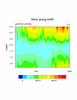
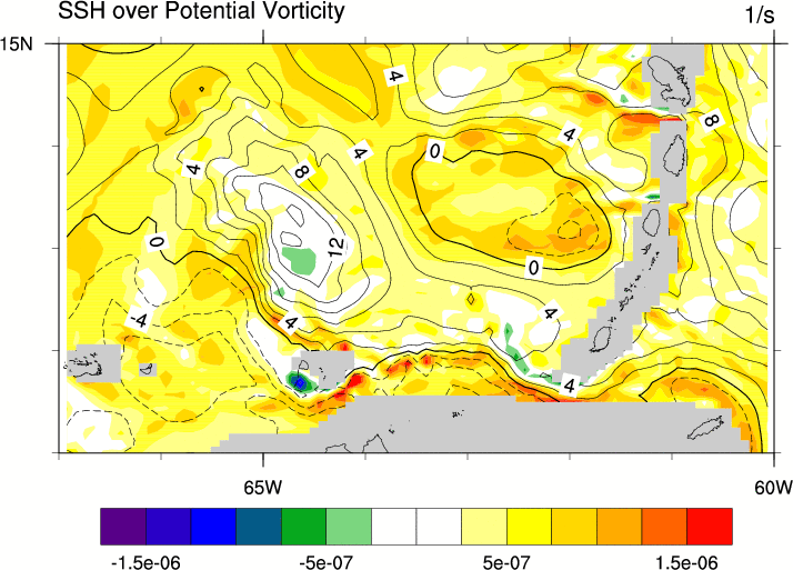nlom_4.ncl: A contour on contour plot.

One way to draw contours on top of contours is to create two separate plots and us overlay to merge the two images. The first plot is created with gsn_csm_contour_map_ce so that it contains the map info. The second plot is created with gsn_csm_contour which contains no map info. The second plot was also passed the resources gsnContourNegLineDashPattern and gsnContourZeroLineThicknessF which will make the zero line double thick and negative values dashed.

Because this plot was a very small region, raster mode was not turned on (the default). This caused one change from example 1, in that an additional resource is required to get the missing value area shaded gray: cnMissingValFillPattern needs to be set to 0 which is solid fill. The default is a hollow fill.