Generally, the larger the array(s) the smoother the derived PDF. Bin sizes of less-than [greater-than] the default number of 25 bins will result in smoother [rougher] plots.
NCL Home>
Application examples>
Data Analysis ||
Data files for some examples
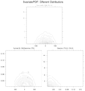
 pdf_1.ncl:
Using the pdfx function,
this example illustrates univariate PDFs from three
variables with three different distributions.
Default settings of parameters are used (eg., 25 bins).
pdf_1.ncl:
Using the pdfx function,
this example illustrates univariate PDFs from three
variables with three different distributions.
Default settings of parameters are used (eg., 25 bins).
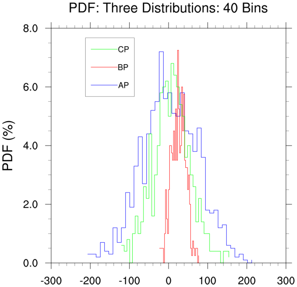
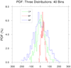 pdf_2.ncl:
This illustrates using a user specified number of bins.
Here, 40 bins are specified. This results in a more ragged
view of the distribution.
Use of the returned bin_center
attributes from three PDFs to place all on
a common x-axis is illustrated. (Minor changes would be required if
the number of bins used had been different.)
The
gsnXYBarChart
and
gsnXYBarChartOutlineOnly
illustrate using a bar style plot.
pdf_2.ncl:
This illustrates using a user specified number of bins.
Here, 40 bins are specified. This results in a more ragged
view of the distribution.
Use of the returned bin_center
attributes from three PDFs to place all on
a common x-axis is illustrated. (Minor changes would be required if
the number of bins used had been different.)
The
gsnXYBarChart
and
gsnXYBarChartOutlineOnly
illustrate using a bar style plot.
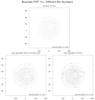
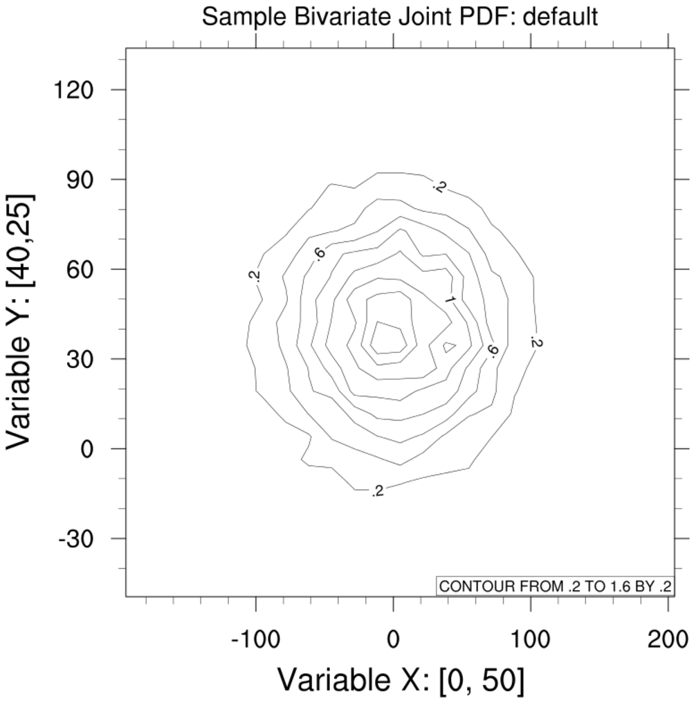
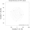 pdf_3.ncl:
Using the pdfxy function,
illustrate a simple bivariate PDF using two variables having normal
distributions.
pdf_3.ncl:
Using the pdfxy function,
illustrate a simple bivariate PDF using two variables having normal
distributions.
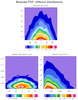
 pdf_4.ncl:
Similar to Example 3 but use different bin numbers.
Given a fixed number of values, the fewer bins used, the smoother
the resulting PDF.
pdf_4.ncl:
Similar to Example 3 but use different bin numbers.
Given a fixed number of values, the fewer bins used, the smoother
the resulting PDF.
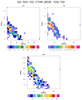
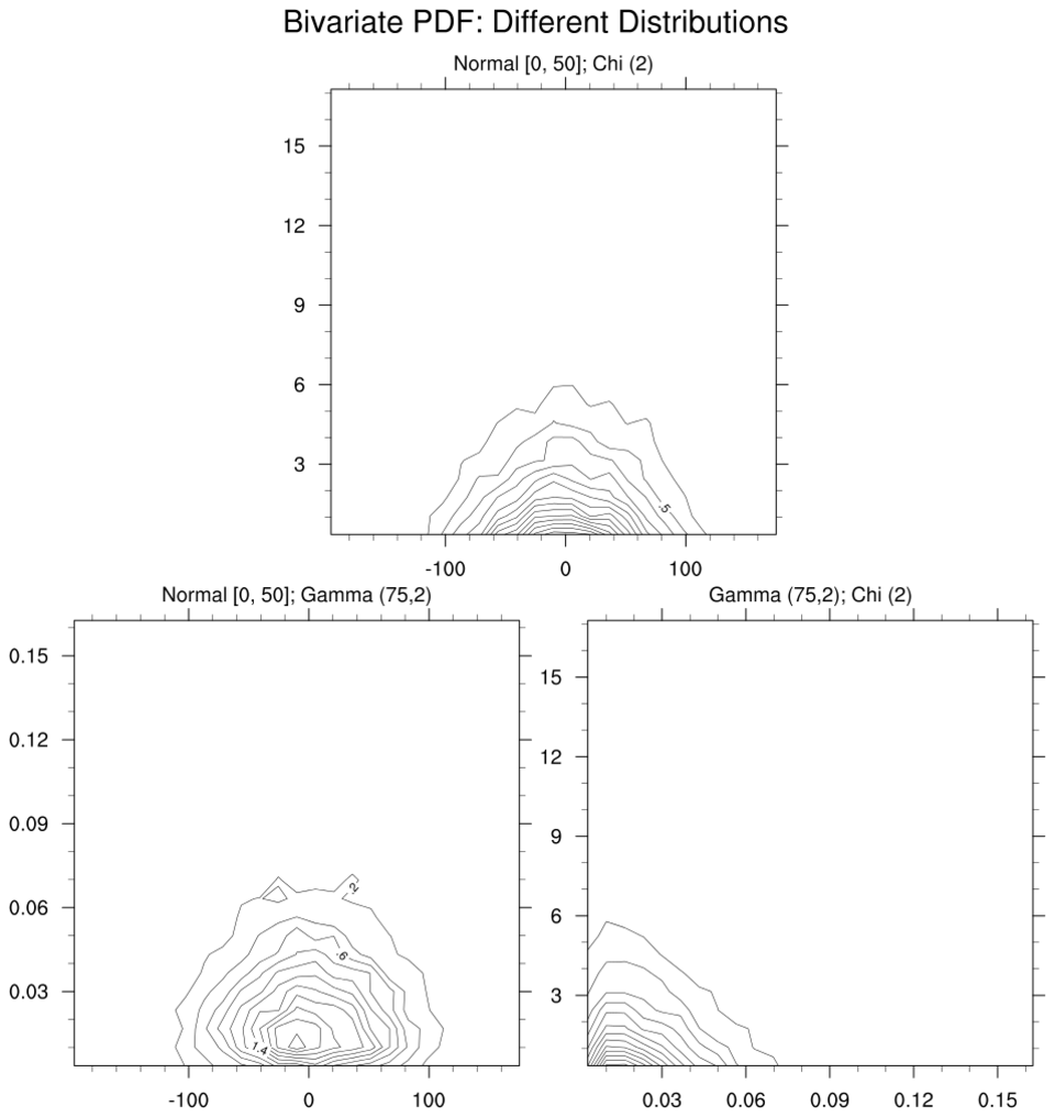
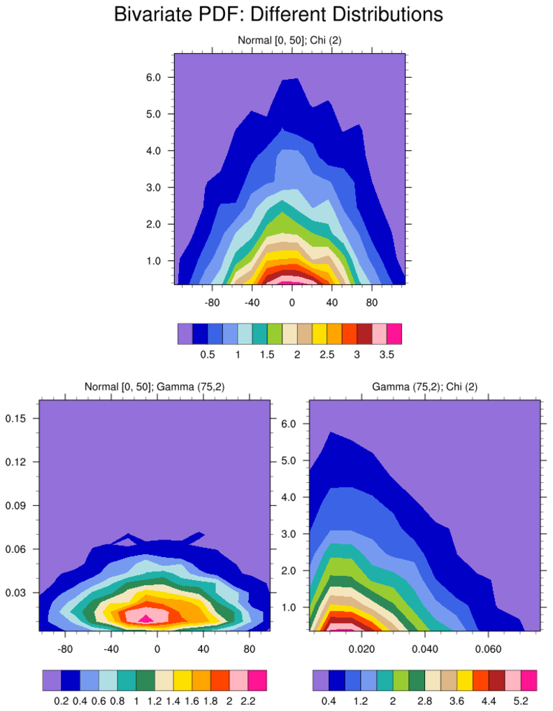
 pdf_5.ncl:
The bivariate distributions of variables from variables with different
univariate distributions will yield different patterns.
Here, the univariate distributions of Example 1 are used
to create bivariate PDFs.
pdf_5.ncl:
The bivariate distributions of variables from variables with different
univariate distributions will yield different patterns.
Here, the univariate distributions of Example 1 are used
to create bivariate PDFs.
 pdf_6.ncl:
Variables that may not be continuous [probabilities=0.0]
may be best viewed via use of "raster" plots. These clearly show
the bin and data resolution.
pdf_6.ncl:
Variables that may not be continuous [probabilities=0.0]
may be best viewed via use of "raster" plots. These clearly show
the bin and data resolution.
Example pages containing: tips | resources | functions/procedures
NCL: Probability Distribution Functions
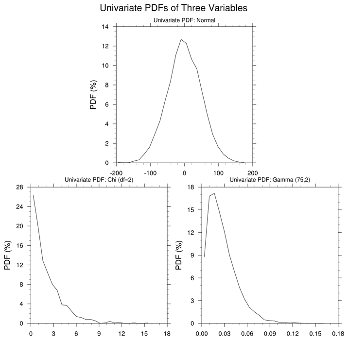
The probability distribution (frequency of occurrence) of an individual
variable, X, may be obtained via the
pdfx function.
Given two variables X and Y, the bivariate
joint probability distribution returned by the pdfxy
function indicates the probability of occurrence defined in terms of both X and Y.
 pdf_1.ncl:
Using the pdfx function,
this example illustrates univariate PDFs from three
variables with three different distributions.
Default settings of parameters are used (eg., 25 bins).
pdf_1.ncl:
Using the pdfx function,
this example illustrates univariate PDFs from three
variables with three different distributions.
Default settings of parameters are used (eg., 25 bins).
 pdf_2.ncl:
This illustrates using a user specified number of bins.
Here, 40 bins are specified. This results in a more ragged
view of the distribution.
Use of the returned bin_center
attributes from three PDFs to place all on
a common x-axis is illustrated. (Minor changes would be required if
the number of bins used had been different.)
The
gsnXYBarChart
and
gsnXYBarChartOutlineOnly
illustrate using a bar style plot.
pdf_2.ncl:
This illustrates using a user specified number of bins.
Here, 40 bins are specified. This results in a more ragged
view of the distribution.
Use of the returned bin_center
attributes from three PDFs to place all on
a common x-axis is illustrated. (Minor changes would be required if
the number of bins used had been different.)
The
gsnXYBarChart
and
gsnXYBarChartOutlineOnly
illustrate using a bar style plot.
 pdf_3.ncl:
Using the pdfxy function,
illustrate a simple bivariate PDF using two variables having normal
distributions.
pdf_3.ncl:
Using the pdfxy function,
illustrate a simple bivariate PDF using two variables having normal
distributions.
 pdf_4.ncl:
Similar to Example 3 but use different bin numbers.
Given a fixed number of values, the fewer bins used, the smoother
the resulting PDF.
pdf_4.ncl:
Similar to Example 3 but use different bin numbers.
Given a fixed number of values, the fewer bins used, the smoother
the resulting PDF.
 pdf_5.ncl:
The bivariate distributions of variables from variables with different
univariate distributions will yield different patterns.
Here, the univariate distributions of Example 1 are used
to create bivariate PDFs.
pdf_5.ncl:
The bivariate distributions of variables from variables with different
univariate distributions will yield different patterns.
Here, the univariate distributions of Example 1 are used
to create bivariate PDFs.
Some tuning of plots may be necessary to focus on regions of interest. Here, the "Gamma/Chi" distributions are highly skewed. There are large areas where the joint probabilites are near or at zero. NCL coordinate subscripting is used to select regions of interest.
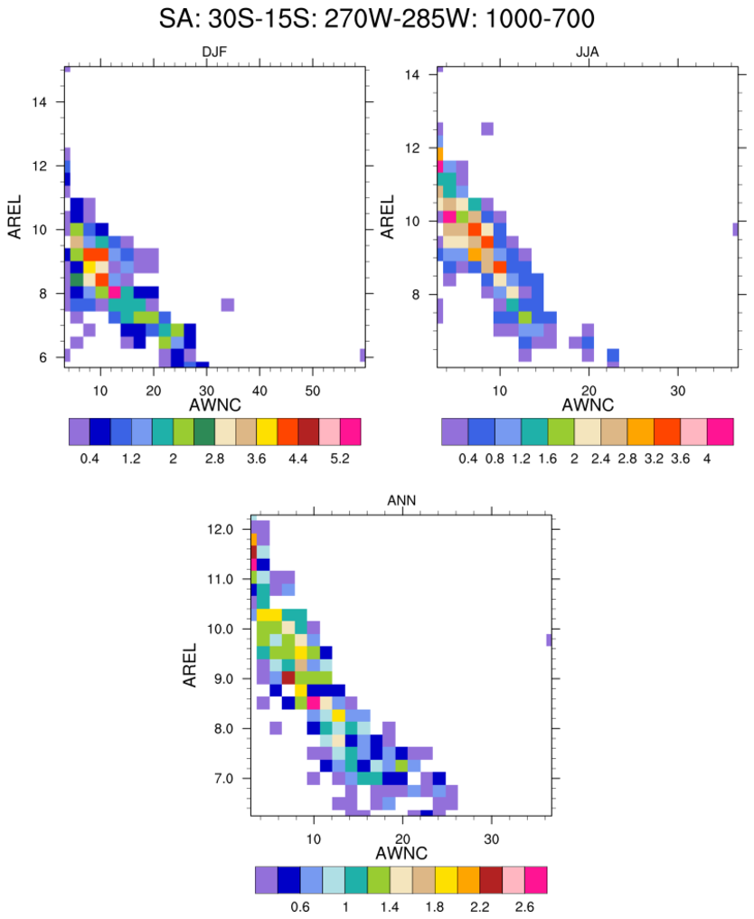
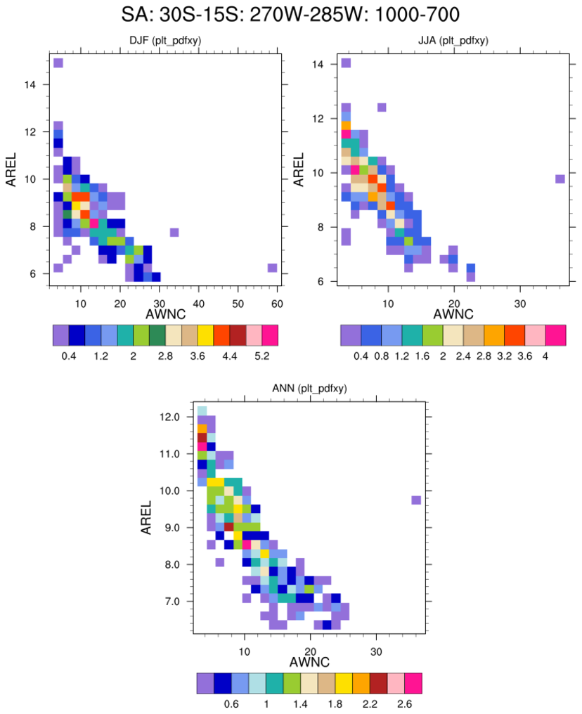 pdf_6.ncl:
Variables that may not be continuous [probabilities=0.0]
may be best viewed via use of "raster" plots. These clearly show
the bin and data resolution.
pdf_6.ncl:
Variables that may not be continuous [probabilities=0.0]
may be best viewed via use of "raster" plots. These clearly show
the bin and data resolution.
Note that using gsn_csm_contour results in the raster bins at the edges being reduced to half width. The use of plt_pdfxy located in the shea_util expands the contour area and allows the edge raster bins to be fully viewed.