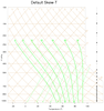
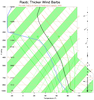
The NCL script "skewt_func.ncl" is included with the NCL distribution.
It is designed to reproduce the "USAF Skew-t, log p diagram (form
dod-wpc 9-16-1)".
It may be loaded via:
load "$NCARG_ROOT/lib/ncarg/nclscripts/csm/skewt_func.ncl"
NCL Home>
Application examples>
Special plots ||
Data files for some examples
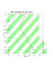
 skewt_1.ncl:
demonstrates the construction of three skew-T plot backgrounds.
The left plot is the default. The center plot was created by setting the
two attributes DrawColAreaFill and DrawHeightScale to "True". The third
plot uses a centigrade scale [DrawFahrenheit = False] and the heights
are indicated in meters [DrawHeightScale=True and
DrawHeightScaleFt=False ].
skewt_1.ncl:
demonstrates the construction of three skew-T plot backgrounds.
The left plot is the default. The center plot was created by setting the
two attributes DrawColAreaFill and DrawHeightScale to "True". The third
plot uses a centigrade scale [DrawFahrenheit = False] and the heights
are indicated in meters [DrawHeightScale=True and
DrawHeightScaleFt=False ].

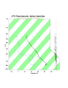
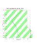
 skewt_2.ncl: Plots
sounding data
on the skew-T plots. Check out those wind barbs! The winds from a (bogus)
pibal are indicated via a different color and thickness.
Printed under the [optional] figure title, are several reference quantities:
skewt_2.ncl: Plots
sounding data
on the skew-T plots. Check out those wind barbs! The winds from a (bogus)
pibal are indicated via a different color and thickness.
Printed under the [optional] figure title, are several reference quantities:
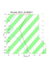
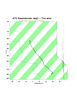 skewt_3.ncl:
Plots sounding data.
The left figure shows the full radiosonde while the right plot "thins"
the number of wind barbs plotted and uses a Centigrade scale. Setting
the Wthin attribute to 3 means plot every third wind barb.
skewt_3.ncl:
Plots sounding data.
The left figure shows the full radiosonde while the right plot "thins"
the number of wind barbs plotted and uses a Centigrade scale. Setting
the Wthin attribute to 3 means plot every third wind barb.
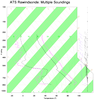 skewt_4.ncl:
This shows how to plot two soundings on the same plot. Basically,
(a) draw the background; (b) draw each sounding upon
the background; (c) advance the frame after all soundings
have been plotted.
Options are used to change colors, line patterns, location of
wind barbs [xpWind] and to thin
the number of wind barbs [Wthin].
The data file is
here.
skewt_4.ncl:
This shows how to plot two soundings on the same plot. Basically,
(a) draw the background; (b) draw each sounding upon
the background; (c) advance the frame after all soundings
have been plotted.
Options are used to change colors, line patterns, location of
wind barbs [xpWind] and to thin
the number of wind barbs [Wthin].
The data file is
here.
 skewt_5.ncl: Panel the skewT
diagrams. This is done via the special "Panel" attribute which you
set to True. This example just repeats the same plot for
demonstrative purposes. Unfortunately, at this time,
The wmvect drawn wind barbs can not be paneled.
The data file is
here.
skewt_5.ncl: Panel the skewT
diagrams. This is done via the special "Panel" attribute which you
set to True. This example just repeats the same plot for
demonstrative purposes. Unfortunately, at this time,
The wmvect drawn wind barbs can not be paneled.
The data file is
here.
 skewt_6.ncl:
Read a RUC (Rapid Update Cycle) GRIB file (here: ruc2anl).
Plot the skewT at the grid point(s) nearest user specified locations.
The getind_latlon2d function
is used to find the nearest locations.
skewt_6.ncl:
Read a RUC (Rapid Update Cycle) GRIB file (here: ruc2anl).
Plot the skewT at the grid point(s) nearest user specified locations.
The getind_latlon2d function
is used to find the nearest locations.
 skewt_7.ncl:
This script accesses upper air netCDF files from the Historical Unidata Internet Data Distribution (IDD)
Global Observational Data archive (ds336.0).
It (a) reads raob data from user specified stations;
(b) plots a skewT of each sounding; (c) creates a simple text (ascii) file containing mandatory
level upper air data. A sample text file (Bermuda_2013030612.ManLevels.txt) follows:
skewt_7.ncl:
This script accesses upper air netCDF files from the Historical Unidata Internet Data Distribution (IDD)
Global Observational Data archive (ds336.0).
It (a) reads raob data from user specified stations;
(b) plots a skewT of each sounding; (c) creates a simple text (ascii) file containing mandatory
level upper air data. A sample text file (Bermuda_2013030612.ManLevels.txt) follows:
 skewt_8.ncl: Manually panel the skewT
diagrams. This allows the wind barbs to be drawn (See Example 5).
For illustration the bottom (Temperature) and left axis (P) titles are turned off and on.
The ascii (text) data file is
here.
skewt_8.ncl: Manually panel the skewT
diagrams. This allows the wind barbs to be drawn (See Example 5).
For illustration the bottom (Temperature) and left axis (P) titles are turned off and on.
The ascii (text) data file is
here.
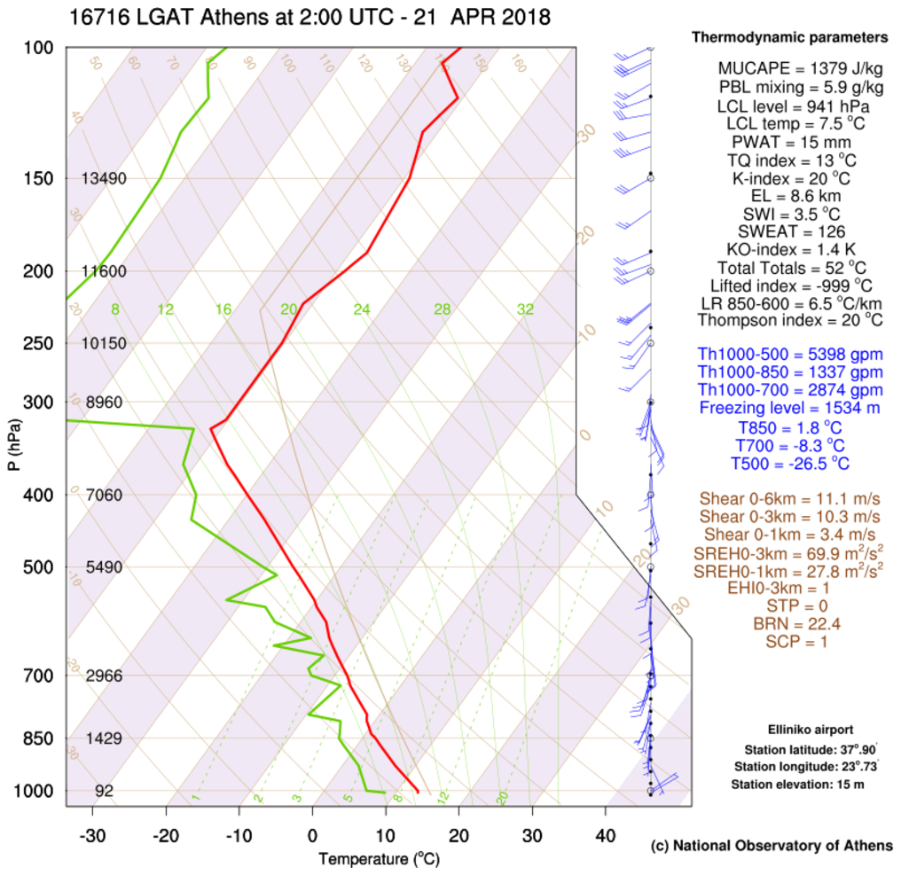
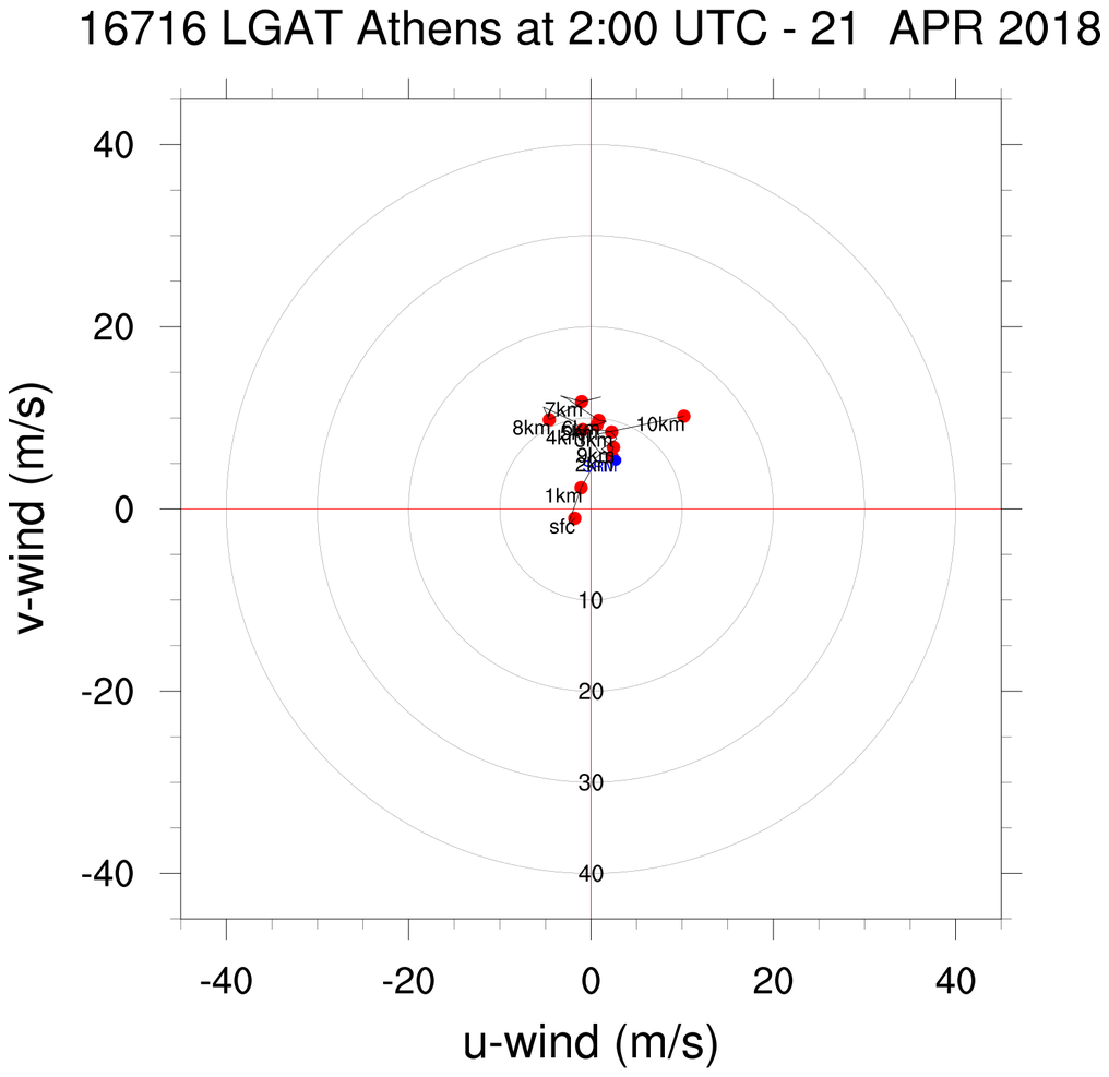
 skewt_9.ncl:
Use scripts donated by Stavros Dafis (National Observatory of Athens/IERSD, Greece;
Polytechnic School of Paris, Laboratory of Dynamic Meteorology (LMD))
to create a hodograph and a skew-T onto which a number of derived quantities are printed.
Click for scripts and data:
skewt_func_dafis.ncl;
hodograph_dafis.ncl;
hodo_cartesian.ncl;
Athens_latest.txt.
skewt_9.ncl:
Use scripts donated by Stavros Dafis (National Observatory of Athens/IERSD, Greece;
Polytechnic School of Paris, Laboratory of Dynamic Meteorology (LMD))
to create a hodograph and a skew-T onto which a number of derived quantities are printed.
Click for scripts and data:
skewt_func_dafis.ncl;
hodograph_dafis.ncl;
hodo_cartesian.ncl;
Athens_latest.txt.
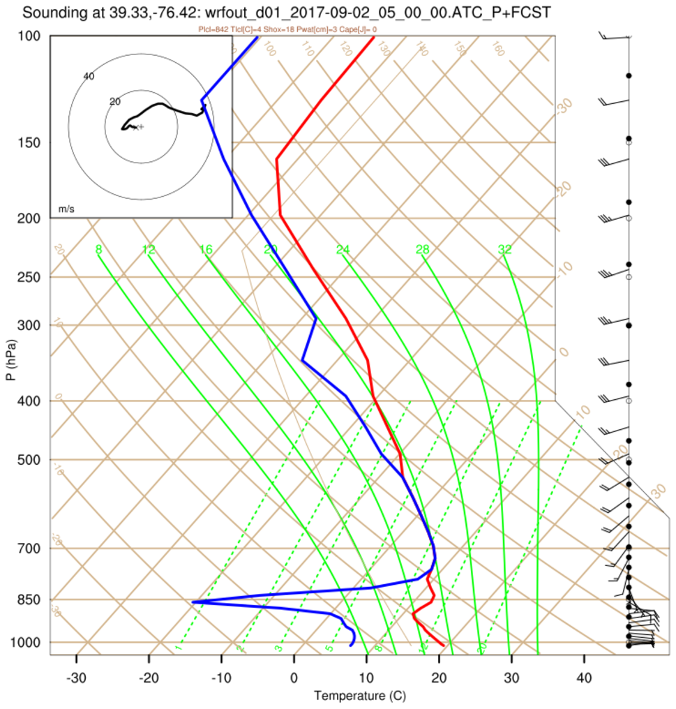
 skewt_10.ncl:
Use a script donated by Joe Grim (RAL; Aviation Applications Program)
to create a single plot containing a hodograph superimposed onto skew-T.
The 'sounding' values are extracted from a WRF netCDF file.
skewt_10.ncl:
Use a script donated by Joe Grim (RAL; Aviation Applications Program)
to create a single plot containing a hodograph superimposed onto skew-T.
The 'sounding' values are extracted from a WRF netCDF file.
Example pages containing:
tips |
resources |
functions/procedures
NCL Graphics: Skew-T
All wind directions/speeds or u-v components are assumed to
reflect conventional meteorological conventions. Missing values,
indicated by the _FillValue attribute, are allowed for any variable.
The user may alter the default behavior of the "skewT_BackGround" and
"skewT_PlotData" functions.
[1] function skewT_BackGround (wks:graphic, Opts:logical)
Setting the "Opts" argument to a variable set to True (eg: opt=True)
allows the user to alter the 'look' of the skewT background.
This is demonstrated in Example 1. The following attributes
may be changed from the default values:
Attribute Default
-------------- ----
DrawIsotherm = True
DrawIsobar = True
DrawMixRatio = True
DrawDryAdiabat = True
DrawMoistAdiabat = True ; aka: saturation or pseudo adibat
DrawWind = True
DrawStandardAtm = True
DrawColLine = True
DrawColAreaFill = False
DrawFahrenheit = True ; Fahrenheit "x" axis
DrawHeightScale = False
DrawHeightScaleFt = True ;default is feet [otherwise km]
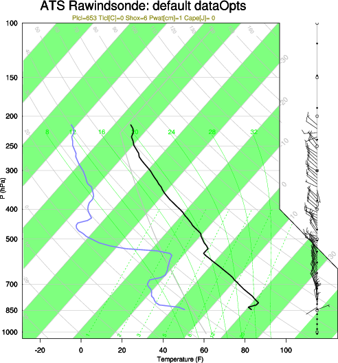
[2] function skewT_PlotData (wks:graphic ,skewt_bkgd:graphic \
,P[*]:numeric ,TC[*]:numeric \
,TDC[*]:numeric ,Z[*]:numeric \
,WSPD[*]:numeric,WDIR[*]:numeric \
,dataOpts:logical )
Setting
dataOpts = True
allows various other options. For example:
                                        ; sounding colors
    dataOpts@colTemperature = "black"   ; default -> "Foreground"
    dataOpts@colDewPt       = "green"   ; default -> "RoyalBlue"
    dataOpts@colCape        = "orange"  ; default -> "Red"
                                        ; Winds at Pressure levels
    dataOpts@colWindP       = "black"   ; default -> "Foreground"
                                        ; Winds at geopotential [Z] levels
    dataOpts@colWindZ       = "black"   ; default -> "Foreground"
                                        ; Winds at pibal Height levels
    dataOpts@colWindH       = "black"   ; default -> "Foreground"

                                        ; sounding line patterns
    dataOpts@linePatternTemperature = 2 ; default=1 [solid]
    dataOpts@linePatternDewPt       = 3 ; default=1 [solid]
    dataOpts@linePatternCape        = 8 ; default=1 [solid]

                                        ; "x" location for windbarbs
    dataOpts@xpWind                 =42 ; default=45

                                        ; By default, skewT_PlotData expects
                                        ; wind speed (WSPD) and direction (WDIR).
    dataOpts@WspdWdir      = False      ; Set to False, if u and v are input.
    dataOpts@DrawWindBarbThk = 2.0      ; make wind barbs thicker; default value is 1.0; NCL version 6.4.0
    dataOpts@hemisphere    = "NH"       ; "NH" -  Northern Hemisphere (default)
                                        ; "SH" -  Southern Hemisphere
    dataOpts@Wthin         = 1          ; Plot a subset of the winds. Default =1
                                        ; =1 means every wind barb
                                        ; =5 would mean every 5-th
                                        ;    wind report would be plotted.
PIBAL reports generally consist of winds at height above the surface.
Below let hght,hspd and hdir represent Pibal wind reports:
    hght = (/1000.,3000.,7000.,25000. /)/3.208  ; hgt (M)
    hspd = (/  50.,  27., 123.,   13. /)        ; speed at each height
    hdir = (/  95., 185., 275.,  355. /)        ; direction

    dataOpts@PlotWindH      = True      ; if available, plot winds at height lvls
    dataOpts@HspdHdir       = True      ; wind speed and dir [else: u,v]
    dataOpts@Height         = hght      ; assign height of wind reports
    dataOpts@Hspd           = hspd      ; speed [or u component]
    dataOpts@Hdir           = hdir      ; dir   [or v component]
Version 5.1.0: The information printed at the top of the skewT plot:
   Cape  -  Convective Available Potential Energy [J]
   Pwat  -  Precipitable Water [cm]
   Shox  -  Showalter Index (stability)
   Plcl  -  Pressure of the lifting condensation level [hPa]
   Tlcl  -  Temperature at the lifting condensation level [C]
is returned as attributes of the returned graphic object.
Example: Let skewT be the returned object. The data may be retrieved via:
   cape = skewT@Cape
   pwat = skewT@Pwat
   shox = skewT@Shox
   plcl = skewT@Plcl
   tlcl = skewT@Tlcl
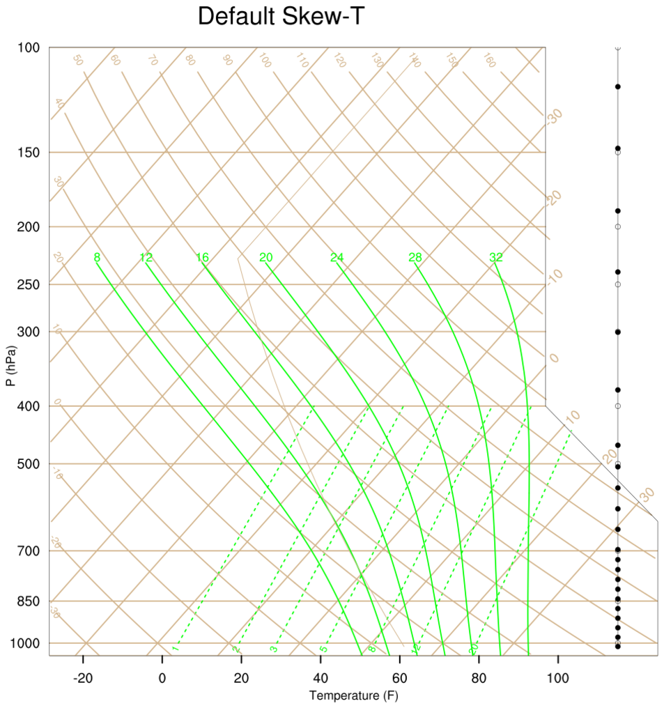
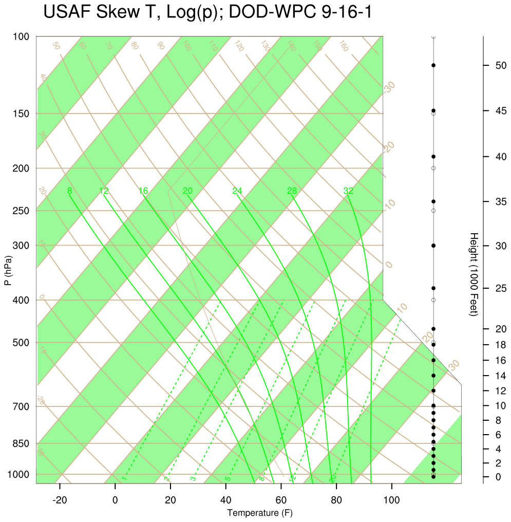
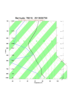
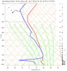
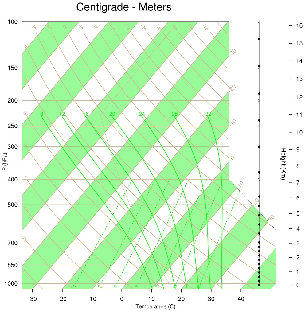 skewt_1.ncl:
demonstrates the construction of three skew-T plot backgrounds.
The left plot is the default. The center plot was created by setting the
two attributes DrawColAreaFill and DrawHeightScale to "True". The third
plot uses a centigrade scale [DrawFahrenheit = False] and the heights
are indicated in meters [DrawHeightScale=True and
DrawHeightScaleFt=False ].
skewt_1.ncl:
demonstrates the construction of three skew-T plot backgrounds.
The left plot is the default. The center plot was created by setting the
two attributes DrawColAreaFill and DrawHeightScale to "True". The third
plot uses a centigrade scale [DrawFahrenheit = False] and the heights
are indicated in meters [DrawHeightScale=True and
DrawHeightScaleFt=False ].
A Python version of this projection is available here.
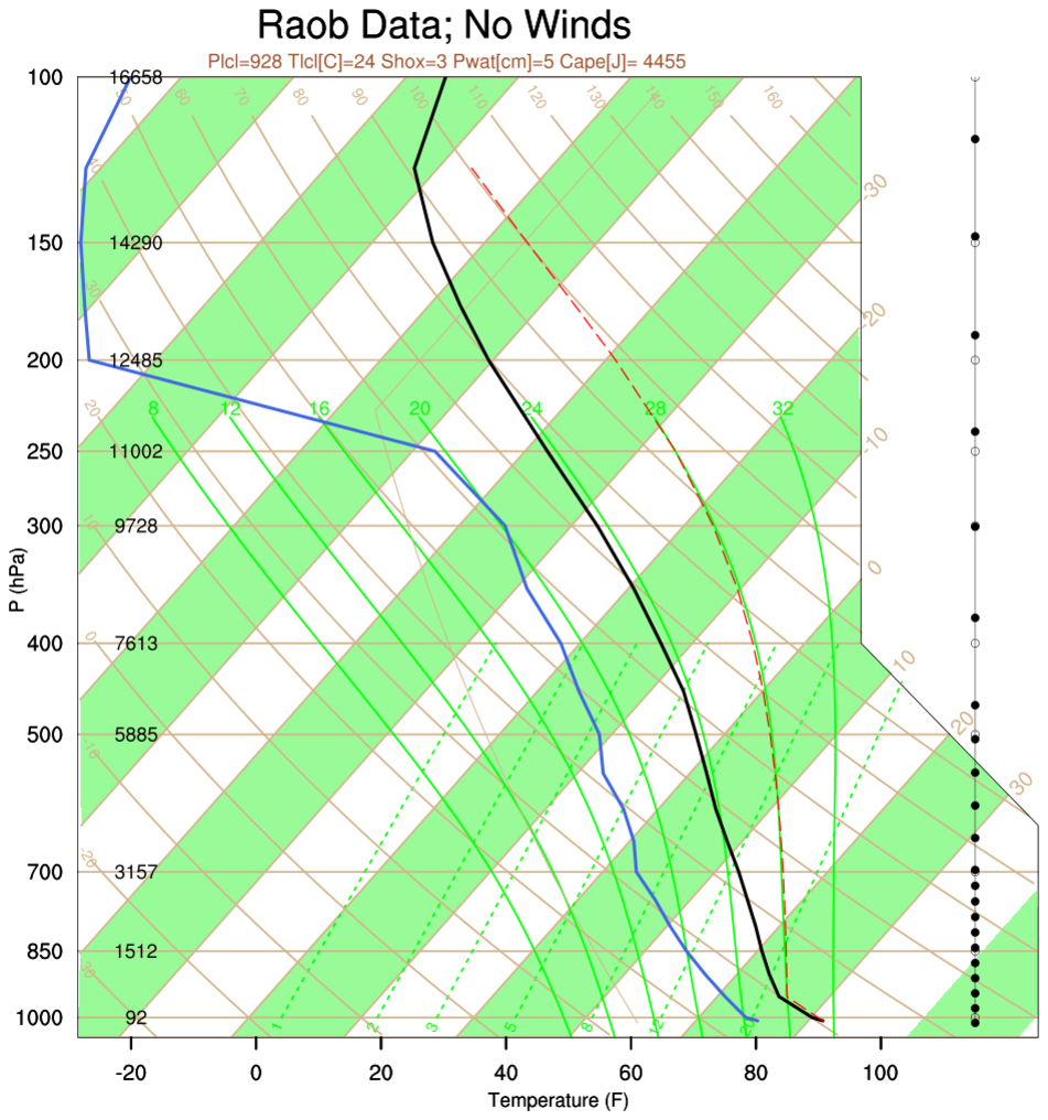
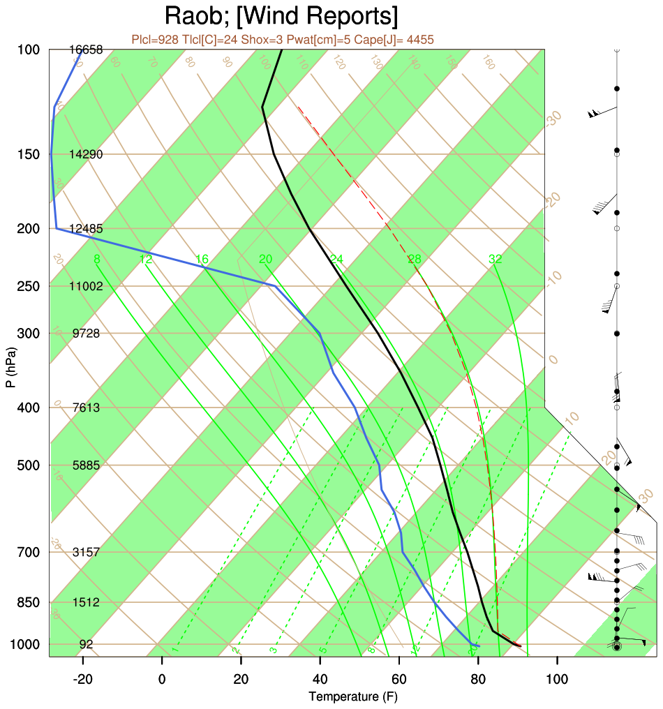
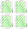
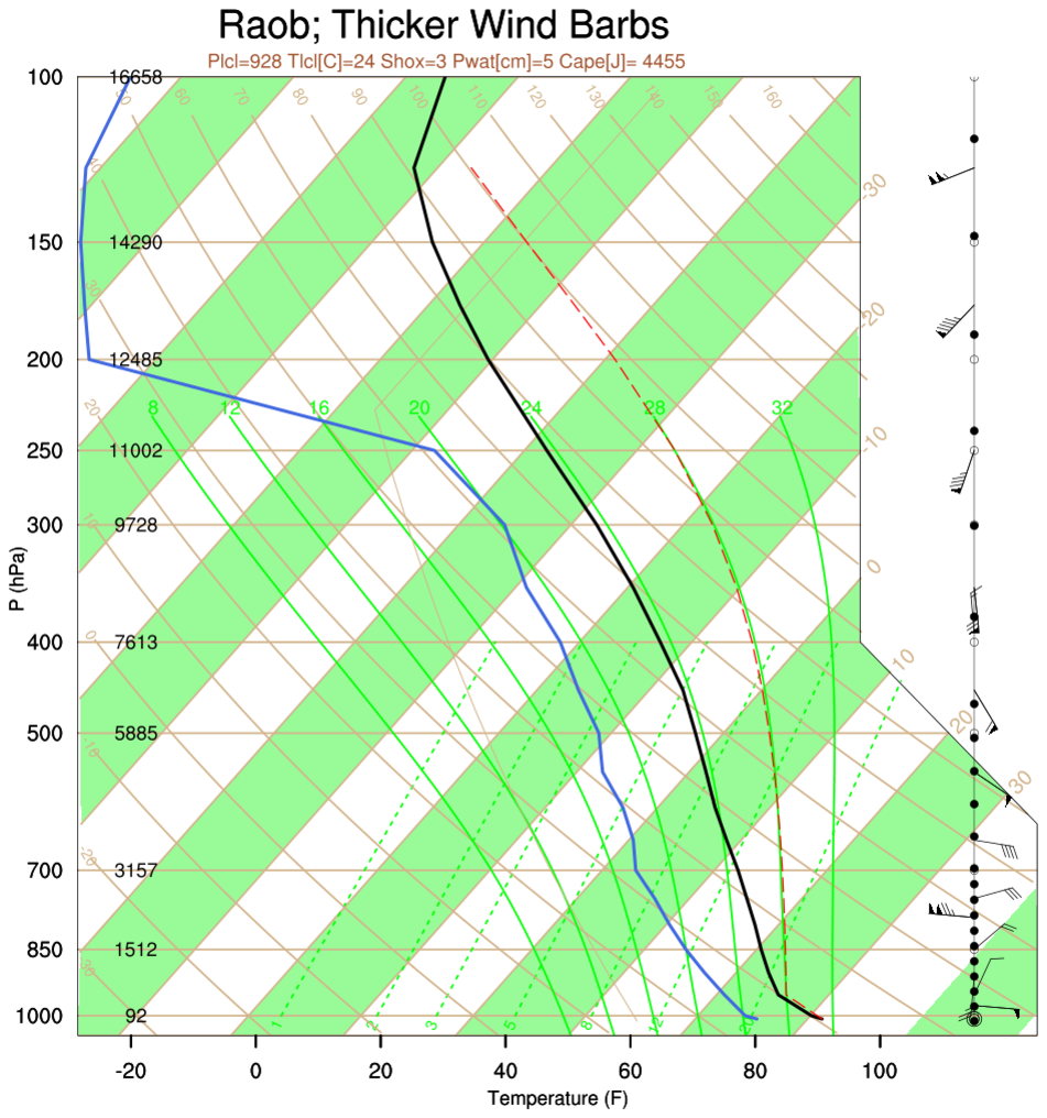 skewt_2.ncl: Plots
sounding data
on the skew-T plots. Check out those wind barbs! The winds from a (bogus)
pibal are indicated via a different color and thickness.
Printed under the [optional] figure title, are several reference quantities:
skewt_2.ncl: Plots
sounding data
on the skew-T plots. Check out those wind barbs! The winds from a (bogus)
pibal are indicated via a different color and thickness.
Printed under the [optional] figure title, are several reference quantities:
    Plcl: Lifting Condensation Level [mb,  hPa]
    Tlcl: Temperature at the LCL
    Shox: Showalter Index
    Pwat: Total Precipitable Water [cm]
    Cape: Convective Available Potential Energy [Joules]
A Python version of skewt_2_2 projection is available here.
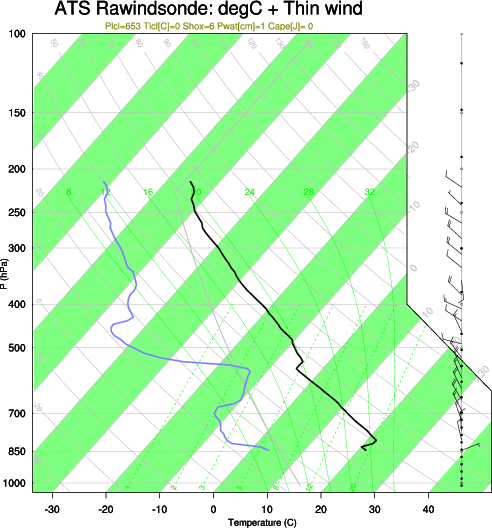 skewt_3.ncl:
Plots sounding data.
The left figure shows the full radiosonde while the right plot "thins"
the number of wind barbs plotted and uses a Centigrade scale. Setting
the Wthin attribute to 3 means plot every third wind barb.
skewt_3.ncl:
Plots sounding data.
The left figure shows the full radiosonde while the right plot "thins"
the number of wind barbs plotted and uses a Centigrade scale. Setting
the Wthin attribute to 3 means plot every third wind barb.
The variables plotted are: T [C], TD [C, dew point temperature], Z [m], WSPD and WDIR [knots or m/s; wind speed and direction]. The only required variable is P [mb; Pressure]. The required order is surface [ie, ground] to top.
A Python version of skewt_3_2 projection is available here.
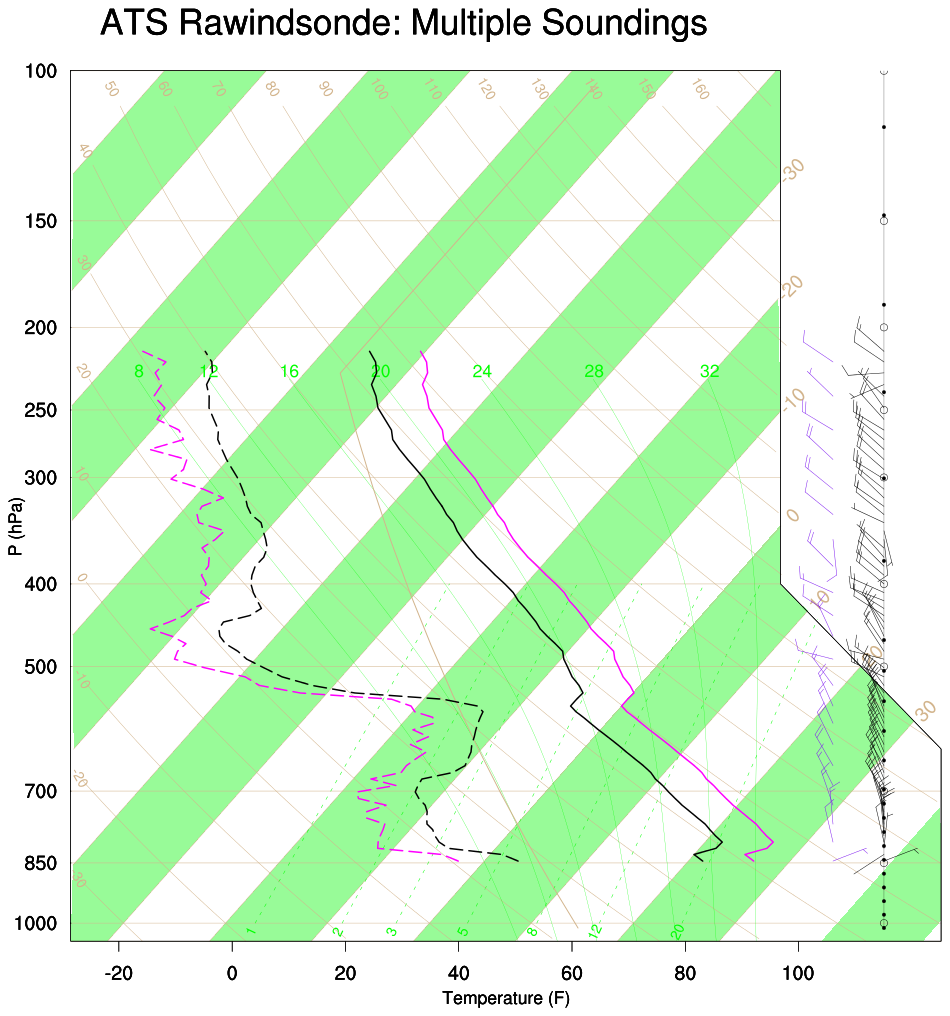 skewt_4.ncl:
This shows how to plot two soundings on the same plot. Basically,
(a) draw the background; (b) draw each sounding upon
the background; (c) advance the frame after all soundings
have been plotted.
Options are used to change colors, line patterns, location of
wind barbs [xpWind] and to thin
the number of wind barbs [Wthin].
The data file is
here.
skewt_4.ncl:
This shows how to plot two soundings on the same plot. Basically,
(a) draw the background; (b) draw each sounding upon
the background; (c) advance the frame after all soundings
have been plotted.
Options are used to change colors, line patterns, location of
wind barbs [xpWind] and to thin
the number of wind barbs [Wthin].
The data file is
here.
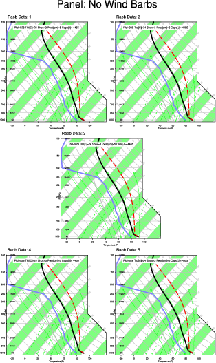 skewt_5.ncl: Panel the skewT
diagrams. This is done via the special "Panel" attribute which you
set to True. This example just repeats the same plot for
demonstrative purposes. Unfortunately, at this time,
The wmvect drawn wind barbs can not be paneled.
The data file is
here.
skewt_5.ncl: Panel the skewT
diagrams. This is done via the special "Panel" attribute which you
set to True. This example just repeats the same plot for
demonstrative purposes. Unfortunately, at this time,
The wmvect drawn wind barbs can not be paneled.
The data file is
here.
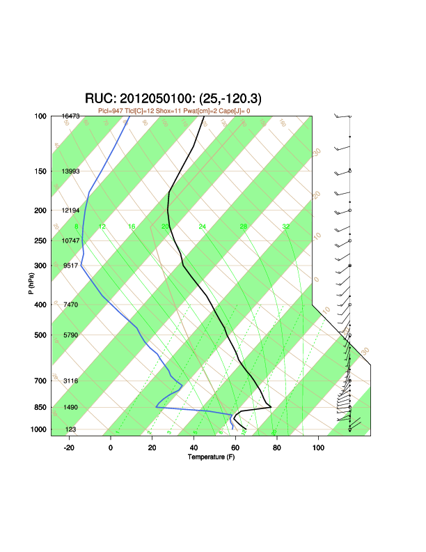
 skewt_6.ncl:
Read a RUC (Rapid Update Cycle) GRIB file (here: ruc2anl).
Plot the skewT at the grid point(s) nearest user specified locations.
The getind_latlon2d function
is used to find the nearest locations.
skewt_6.ncl:
Read a RUC (Rapid Update Cycle) GRIB file (here: ruc2anl).
Plot the skewT at the grid point(s) nearest user specified locations.
The getind_latlon2d function
is used to find the nearest locations.
DSS Example: NCAR's Data Support Section has created an
which plots a skewT diagram with
NCEP ADP Global Upper Air and Surface (PREPBUFR and NetCDF formats) Weather Observations.
The keywords station_icao and station_synop should represent the same observing station. Thus, for Denver Stapleton, the values would be station_icao = KDNR and station_synop = 72469. Since the program is plotting a skew-T log p diagram, the input NetCDF file should contain data from a valid synoptic observing station where radiosondes are launched, and that the input time is either 00 or 12Z (the synoptic times when radiosondes are launched). The script assumes the user knows this beforehand and make the appropriate selection.
Since the program is plotting a skew-T log p diagram, the input NetCDF file should contain ADPUPA observational data from a valid synoptic observing station where radiosondes are launched, and that the input time is either 00 or 12Z (the synoptic times when radiosondes are launched).
The DSS also provide IDL software to create a skewT.
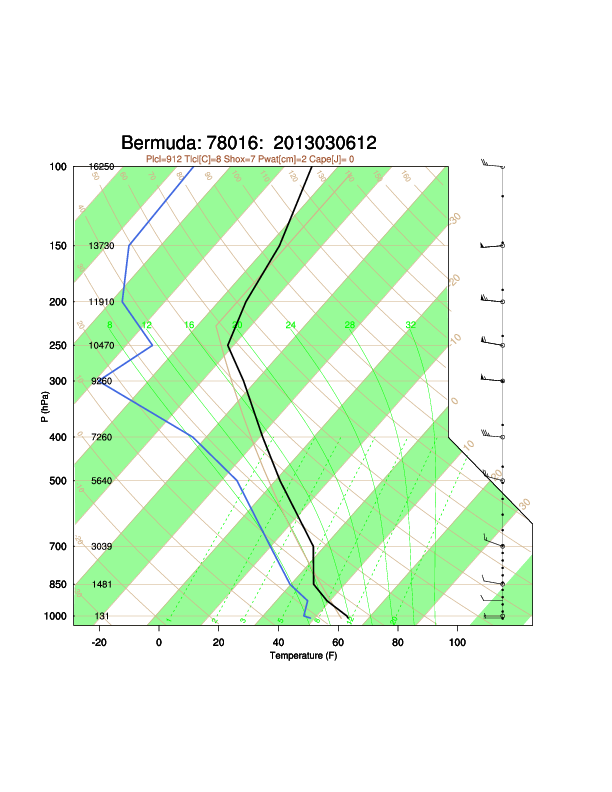
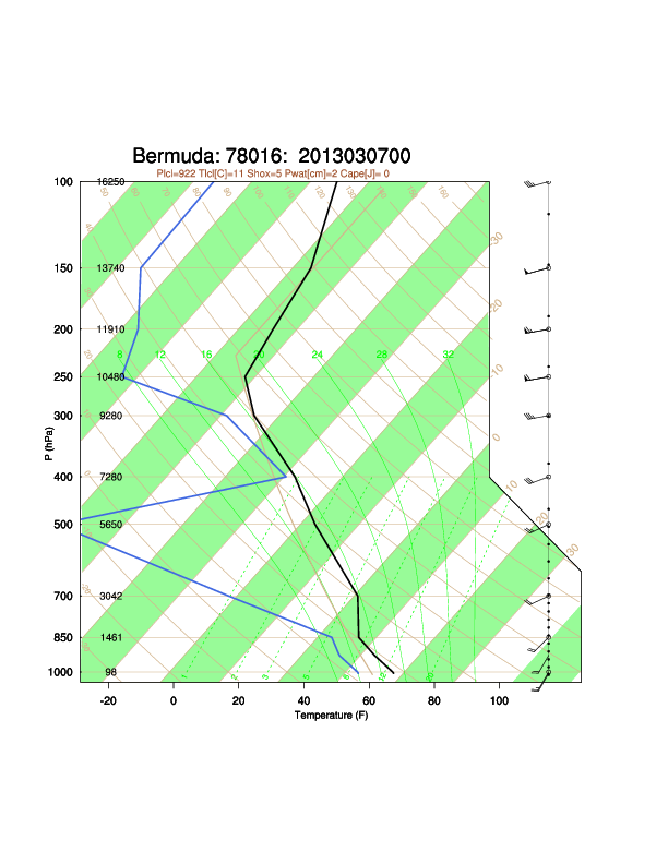
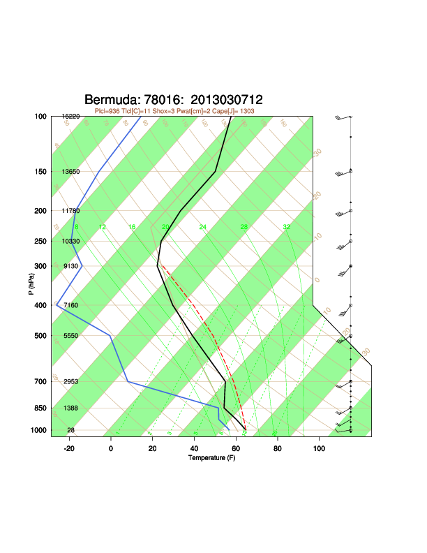 skewt_7.ncl:
This script accesses upper air netCDF files from the Historical Unidata Internet Data Distribution (IDD)
Global Observational Data archive (ds336.0).
It (a) reads raob data from user specified stations;
(b) plots a skewT of each sounding; (c) creates a simple text (ascii) file containing mandatory
level upper air data. A sample text file (Bermuda_2013030612.ManLevels.txt) follows:
skewt_7.ncl:
This script accesses upper air netCDF files from the Historical Unidata Internet Data Distribution (IDD)
Global Observational Data archive (ds336.0).
It (a) reads raob data from user specified stations;
(b) plots a skewT of each sounding; (c) creates a simple text (ascii) file containing mandatory
level upper air data. A sample text file (Bermuda_2013030612.ManLevels.txt) follows:
     P      HGT     T      TDEW    WSPD    WDIR
    mb       m      C        C      m/s
   1011       6    16.2     9.2     5.7     270
   1000     131    15.6     7.6     6.7     270
    925     786     9.4     5.8     9.3     270
    850    1481     4.2    -0.2    11.8     280
    700    3039    -2.1   -10.1    14.4     290
    500    5640   -19.1   -27.1    24.2     285
    400    7260   -29.5   -42.5    35.0     275
    300    9260   -42.3   -69.3    55.6     275
    250   10470   -51.1   -65.1    58.1     280
    200   11910   -54.9   -77.9    62.8     275
    150   13730   -57.9   -85.9    51.4     265
    100   16250   -64.9   -86.9    26.2     275
     70   18400   -64.3   -86.3    24.7     260
     50   20460   -63.5   -86.5    13.9     255
  99999   99999 99999.0 99999.0 99999.0   99999
[snip]
  99999   99999 99999.0 99999.0 99999.0   99999
The script will also plot wind barbs for significant wind levels ('sigW') if there
are any on the file. In this case, none were available.
NOTE: [1] The units of the time variable ('synTime') contain parentheses. These are non-standard. The script assigns the correct units. [2] The variable 'numSigW' has no attribute which indicates a missing value (ie, missing_value or _FillValue). The script assigns the appripriate _FillValue. A few other variables on the file have missing _FillValue attributes.
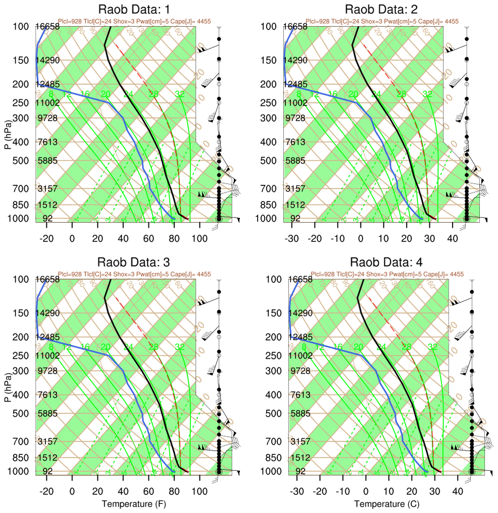 skewt_8.ncl: Manually panel the skewT
diagrams. This allows the wind barbs to be drawn (See Example 5).
For illustration the bottom (Temperature) and left axis (P) titles are turned off and on.
The ascii (text) data file is
here.
skewt_8.ncl: Manually panel the skewT
diagrams. This allows the wind barbs to be drawn (See Example 5).
For illustration the bottom (Temperature) and left axis (P) titles are turned off and on.
The ascii (text) data file is
here.
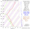
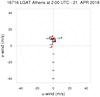
 skewt_9.ncl:
Use scripts donated by Stavros Dafis (National Observatory of Athens/IERSD, Greece;
Polytechnic School of Paris, Laboratory of Dynamic Meteorology (LMD))
to create a hodograph and a skew-T onto which a number of derived quantities are printed.
Click for scripts and data:
skewt_func_dafis.ncl;
hodograph_dafis.ncl;
hodo_cartesian.ncl;
Athens_latest.txt.
skewt_9.ncl:
Use scripts donated by Stavros Dafis (National Observatory of Athens/IERSD, Greece;
Polytechnic School of Paris, Laboratory of Dynamic Meteorology (LMD))
to create a hodograph and a skew-T onto which a number of derived quantities are printed.
Click for scripts and data:
skewt_func_dafis.ncl;
hodograph_dafis.ncl;
hodo_cartesian.ncl;
Athens_latest.txt.
 skewt_10.ncl:
Use a script donated by Joe Grim (RAL; Aviation Applications Program)
to create a single plot containing a hodograph superimposed onto skew-T.
The 'sounding' values are extracted from a WRF netCDF file.
skewt_10.ncl:
Use a script donated by Joe Grim (RAL; Aviation Applications Program)
to create a single plot containing a hodograph superimposed onto skew-T.
The 'sounding' values are extracted from a WRF netCDF file.