NCL Home>
Application examples>
Plot techniques
NCL Graphics: Text (adding to a plot)
There are many ways you can manipulate text, including:
- formatting the string (for floating point or integers) using
sprinti and/or sprintf
- changing the font (via xxYYYYFont resources, or a function code)
- making it larger (via xxYYYYFontHeightF resources)
- changing the color (via xxYYYYFontColor resources)
Function codes:
There are many
fonts/character
sets in NCL (e.g. Greek). You change between sets by using
a function code.
The default code is a ":", but since this is a character that people
often put into their strings, we recommend changing that to a non-used
character like a "~" (in V6.1.0 of NCL and later, the default function
code is a "~"). You can change this on the fly or in
your .hluresfile.
To add a Greek character, use fonts/character set
F33 (e.g. ~F33~s is a sigma). See example xy_10.ncl for details.
To superscript: ~S~
To subscript: ~B~
 text_add_1.ncl
 /
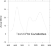
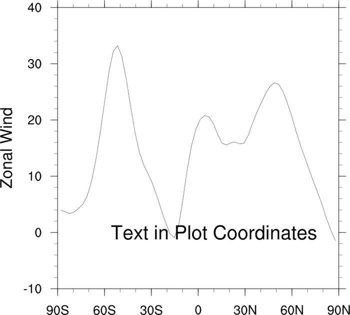
text_1.ncl: Adds text to a plot using
plot coordinates
There are two different ways you can put text on an existing plot
using plot coordinates: using
the gsn_add_text function
(text_add_1.ncl), or
the gsn_text
procedure text_1.ncl).
The gsn_add_text function is usually
the better one to use. It actually attaches the text the plot, so if
you resize the plot, the text will automatically resize (see example
text_9.ncl below). This is especially important if
you plan to panel the text later. It's a little more work, because you
have to call draw on the plot in order to see the
text. With the
gsn_text procedure, you see the
text right away.
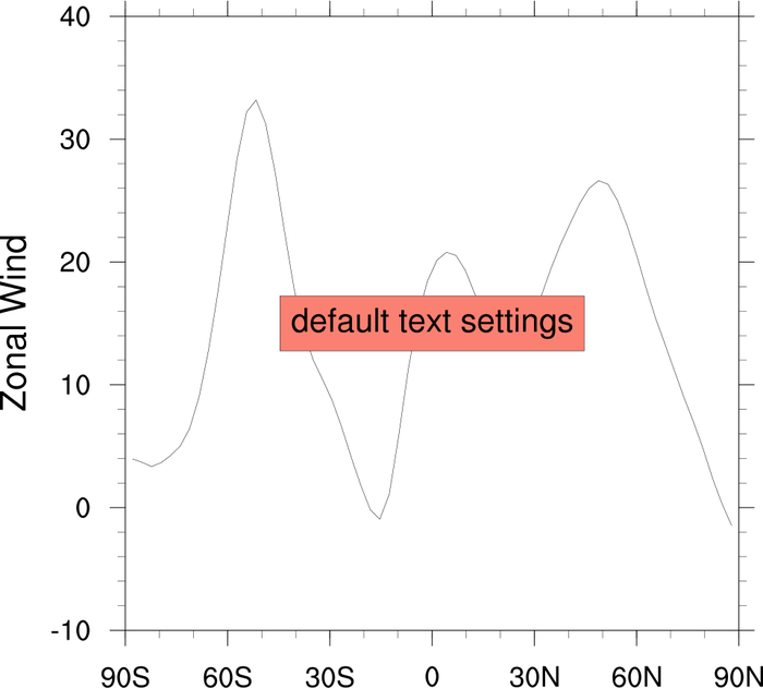
The default added text size is too large, so we have made it smaller
using txFontHeightF. You could also
change the color etc of the text here as well.
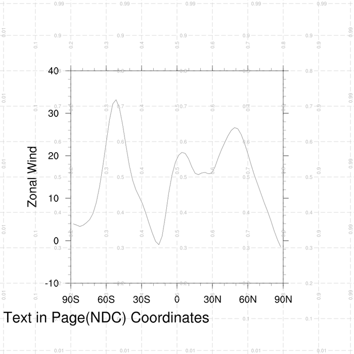
 text_2.ncl
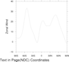
: Adds text to a plot using
page (ndc) coordinates.
gsn_text_ndc is the plot interface
that adds text to an already created plot using page
coordinates. Note: page coordinates are normalized. They go from
0->1.0 in both directions.
 text_3.ncl
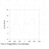
: Can be difficult to
determine the NDC coordinates of a page. Adam Phillips created a nifty
function that draws an NDC grid on a plot. This allows the user to
determine their text placement in fewer iterations.
drawNDCGrid draws the grid.
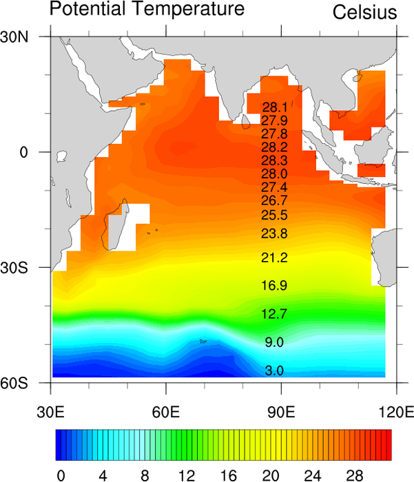
 text_4.ncl
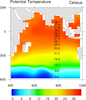
: Demonstrates adding data
values to a contour plot.
sprintf is the function that formats the text output.
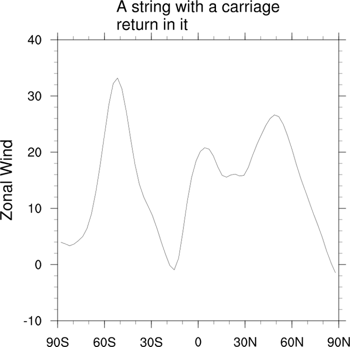
 text_5.ncl
: Demonstrates adding
a carriage return to a text string.
The ~C~ will put a carriage return in a text string. By default
it is left justified. If you need it centered, you will have to
add spaces.
The ~ is a function code. The default function code is a colon (:),
but we have changed this to a ~ in our
.hluresfile
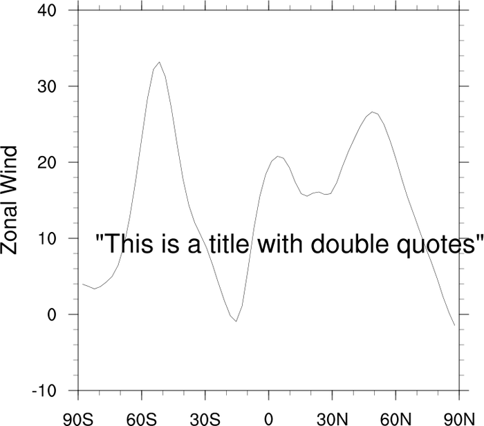
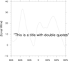 text_6.ncl
: Demonstrates how to
put a double quote into a text string.
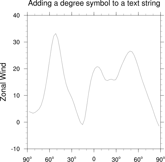
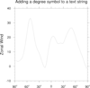 text_7.ncl
: Demonstrates how to
put a degree symbol into a string.
 text_9.ncl
: This example shows how to
use
gsn_create_text to create text
strings and
gsn_add_annotation to attach text items to a
plot.
By attaching the strings, they will get resized if you resize the plot
(see last frame).
The default is to put the string in the center of the plot. In order
to change how the string is positioned, you can set some annotation
resources: amParallelPosF,
amOrthogonalPosF, and amJust. The amParallelPosF and amOrthogonalPosF resources indicate
where, relative to the plot's boundaries, to position the string, and
the amJust resource indicates
which one of nine possible locations on the string ("CenterCenter",
"TopCenter", "TopRight", "CenterRight", "BottomRight", "BottomCenter",
"BottomLeft", "CenterLeft", "TopLeft") about which the string is
positioned.
See example text_18.ncl below for a similar example
that adds to strings to four plots and panels them.
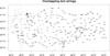
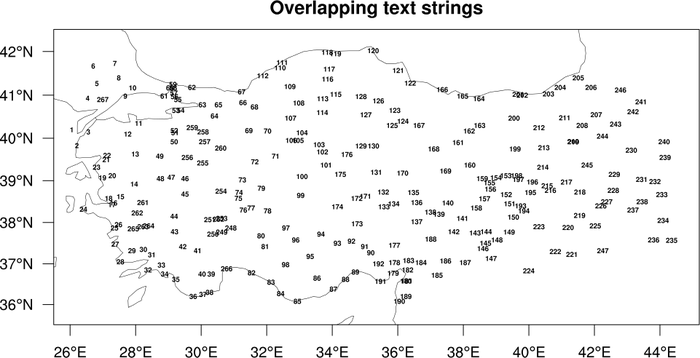
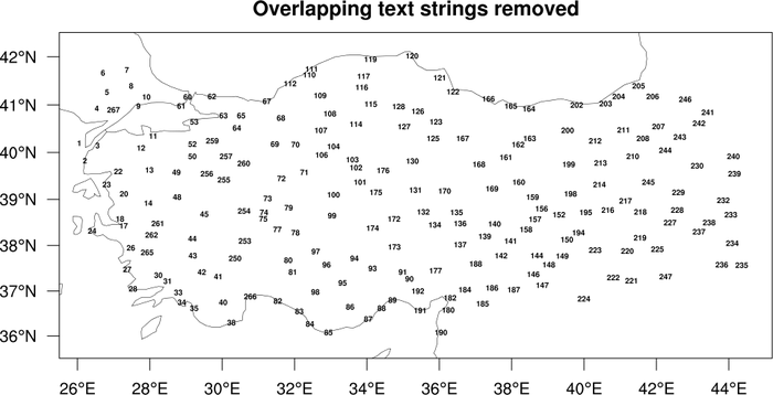
 text_10.ncl
: This example shows how
to use
gsn_add_text to add lots of
strings to a map plot, and then how to determine which ones overlay
other strings so you can remove them.
You can download the small istasyontablosu_son.txt data
file for this example. Thanks to Ozan Mert Gokturk for providing the
data file and the inspiration for this example.
This example is similar to "text_17.ncl" below, which removes strings
that fall on the plot's borders.
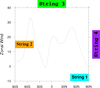
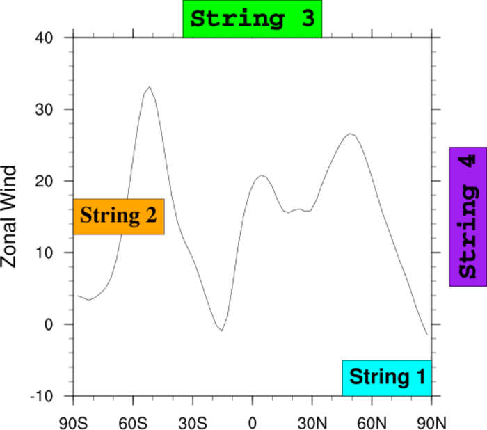
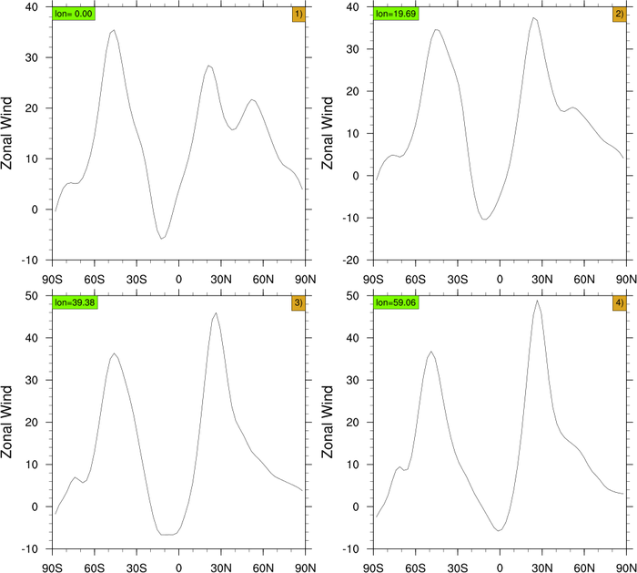
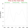 text_12.ncl
: This example shows how
to add three subtitles at the top of any plot, mimicing the subtitles
you get in the
gsn_csm
functions.
The gsn_create_text and gsn_add_annotation functions are used to
create and attach the text strings.
The key to getting the strings to be either left-justified,
right-justified, or centered is to use a combination of the amJust and amParallelPosF resources. You also need
to set amOrthogonalPosF to some
small value to move the strings away from the top edge (tickmarks) of
the plot. This value should be the same for all three strings, in
order to keep them lined up.
- Left-justified string:
- amJust = "BottomLeft"
amParallelPosF = -0.5
- Centered string:
- amJust = "BottomCenter"
amParallelPosF = 0.0
- Right-justified string:
- amJust = "BottomRight"
amParallelPosF = 0.5
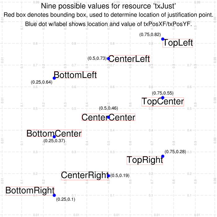
 text_13.ncl
: This example shows how
to use the
txJust resource to align
text.
To place text using a gsn_text* routine, you
specify X and Y positions of the text box that encloses the string.
By default, the text string box is centered about that X,Y position,
unless you set txJust to one of the
other eight allowed values: "BottomRight", "CenterRight", "TopRight",
"BottomCenter", "TopCenter", "BottomLeft", "CenterLeft", or
"TopLeft". ("CenterCenter" is the default.)
 text_14.ncl
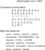
: This example shows how
to use
text function
codes to draw accented characters like the umlaut. This is
done using the H and V function codes that allow you to do small
vertical and horizontal moves as you are drawing text.
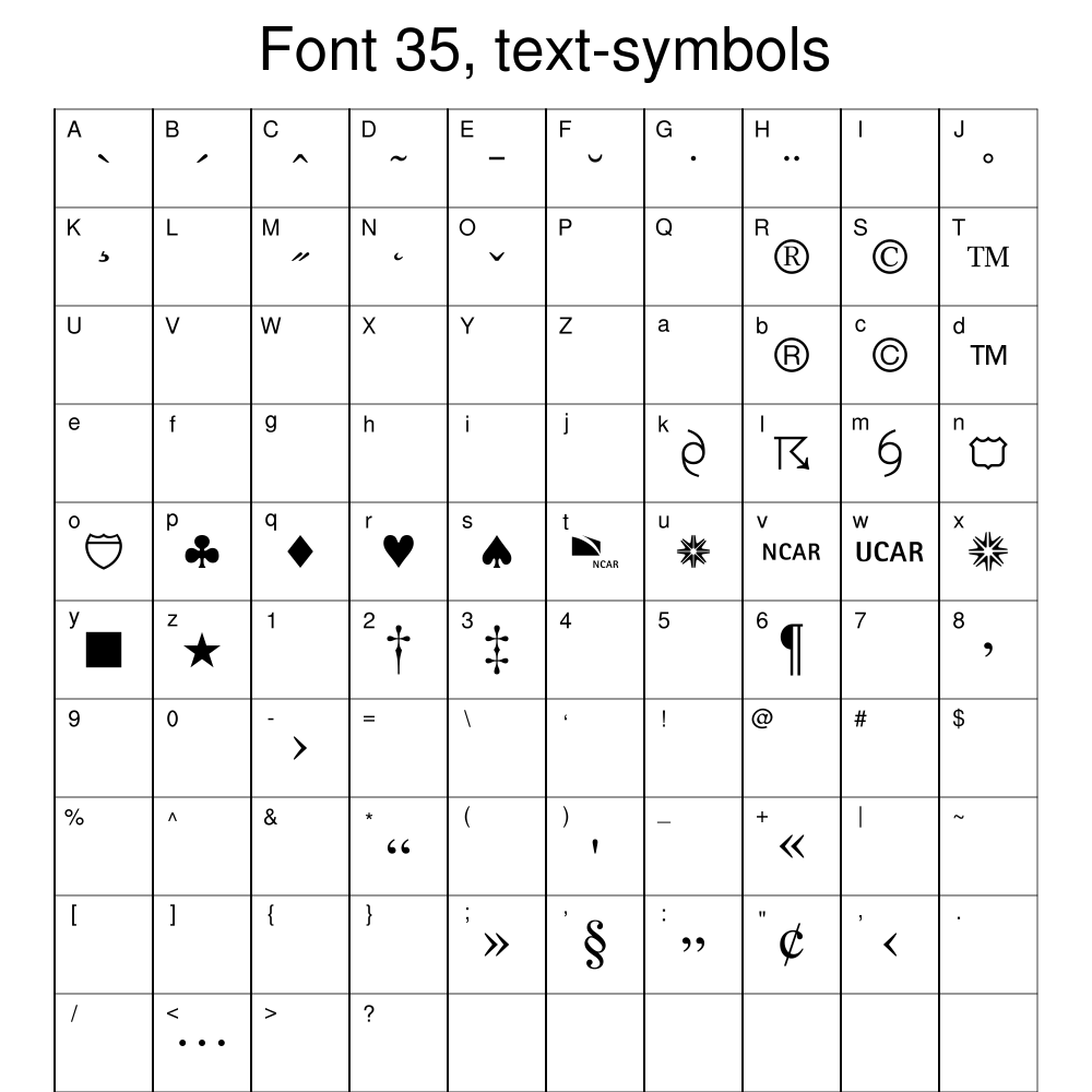
For example, the double dots in the umlaut are drawn by using
character "H" from font
table 35, and a series of horizontal and vertical moves to put
the dots over the desired character.
This script was contributed by Mateus da Silva Teixeira from IPMet.
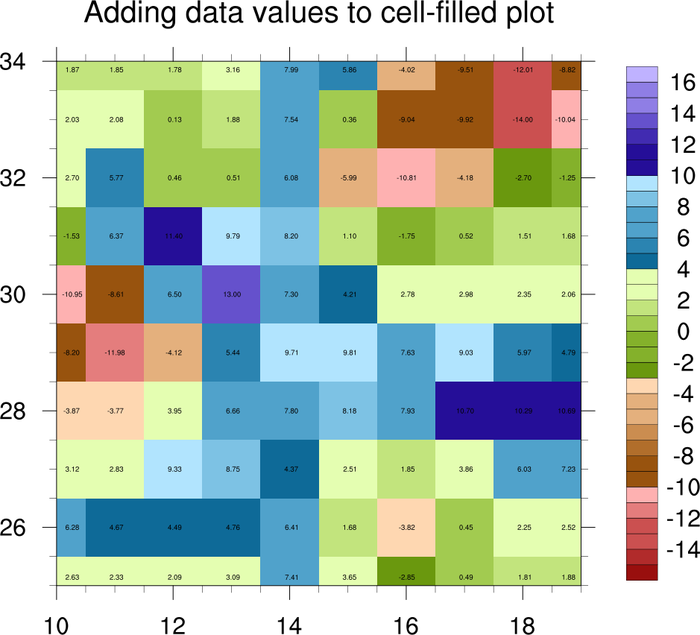
 text_15.ncl
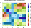
: This example shows how
to use
gsn_add_text to add
data values to an existing cell-filled contour plot.
The txJust resource is set to
"CenterCenter", unless the text string is on one of the four edges of
the plot.
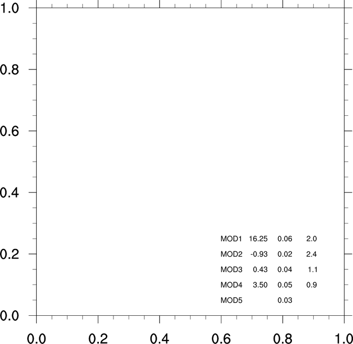
 text_16.ncl
: This example shows how
to use
sprintf in conjunction with
txJust to make sure text strings
with floating point numbers line up at their decimal points.
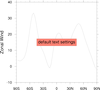
 newcolor_2.ncl
: This example
shows how to create a text string that is highly transparent by
setting the
txFontOpacityF resource
to 0.10. A value of 1.0 means fully opaque.
This capability was added in
NCL version 6.1.0.
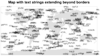
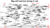
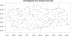
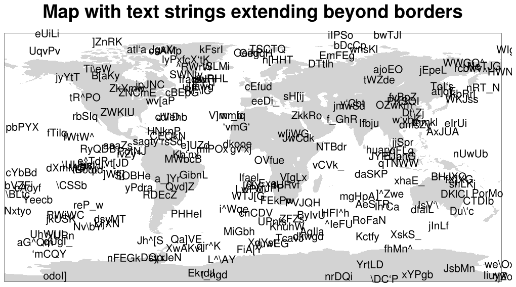
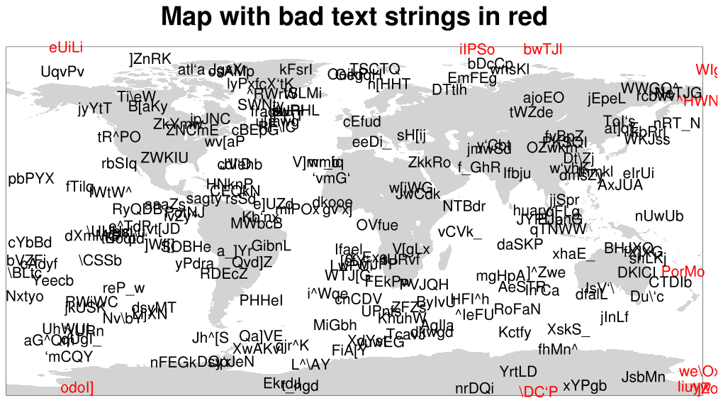
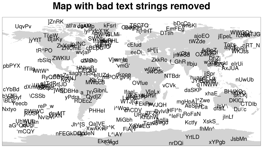
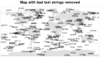 text_17.ncl
: This example shows how
to remove text strings that were added to a map that fall outside
the map's borders. Since there's no way to clip these strings,
you need to use
NhlRemoveAnnotation to
remove the offending text strings.
This example shows three versions of the map: the original plot with the
"bad" strings, the plot with the "bad" strings drawn in a different
color, and the plot with the "bad" strings removed.
This example is similar to "text_10.ncl", which shows how to remove
overlapping strings.
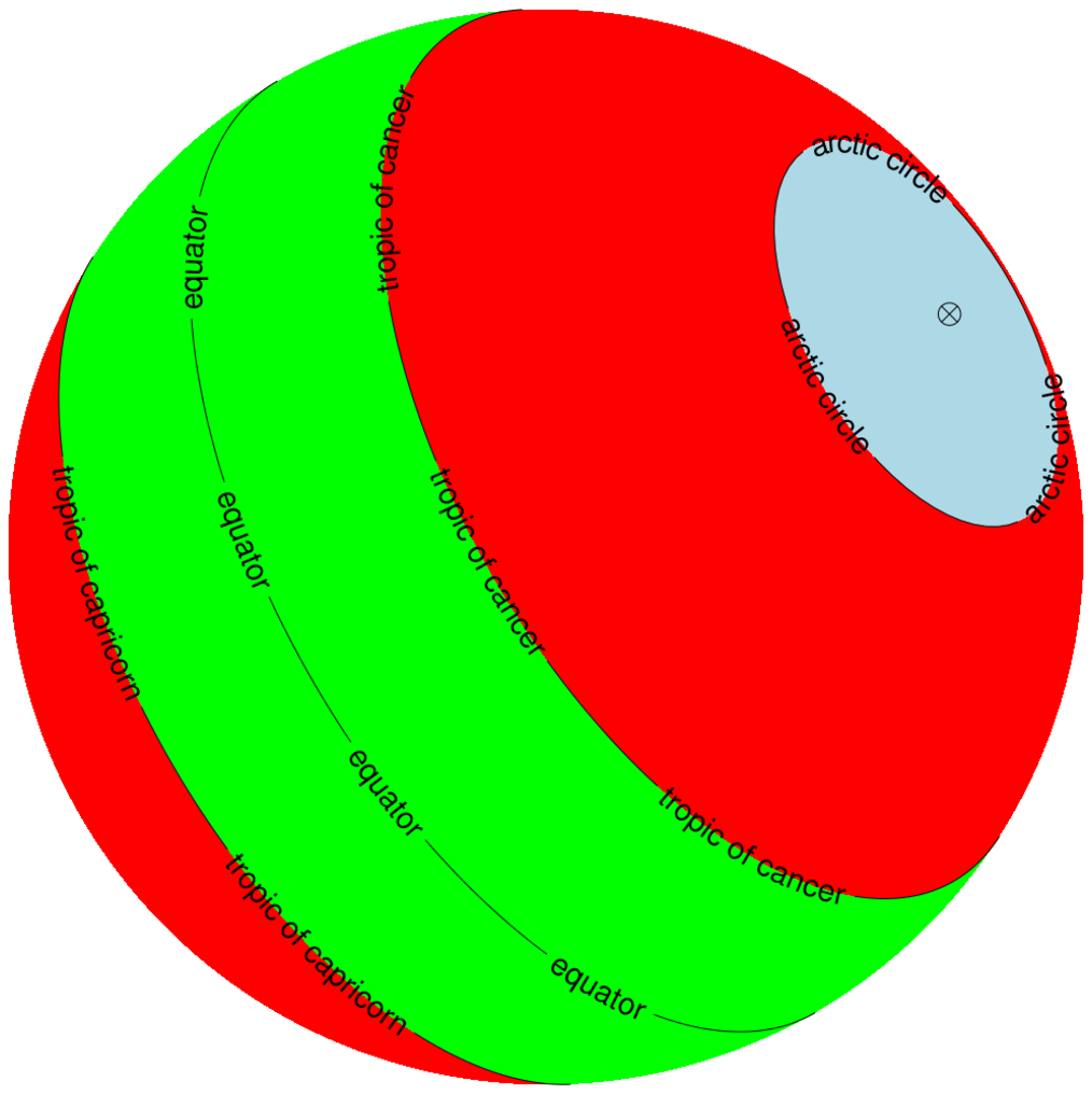
 text_19.ncl
: This example shows how
to draw text strings on a map that follow the curve of a lat/lon
line.
The key is to use
gsn_polyline or
gsn_add_polyline to define the
lat/lon line, and set the special
resources gsLineLabelString
resource to the desired string.
Note: we discovered a bug in NCL that causes this script not to
work with NCL versions 6.2.0, 6.2.1, or 6.3.0. We have a ticket on
this (NCL-2262), and hope to fix it for version 6.4.0.
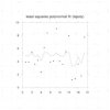
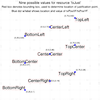
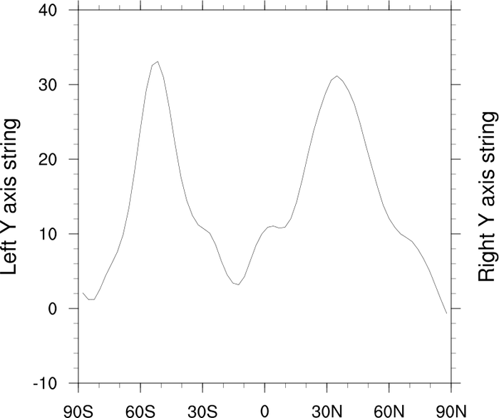
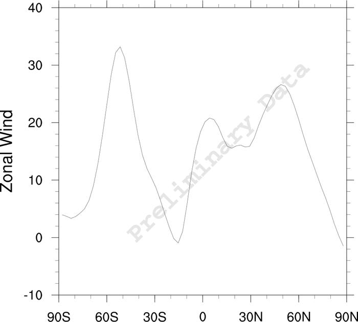
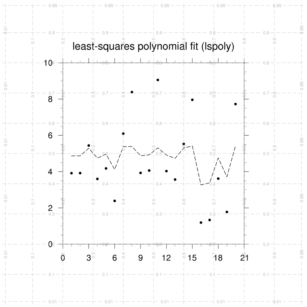
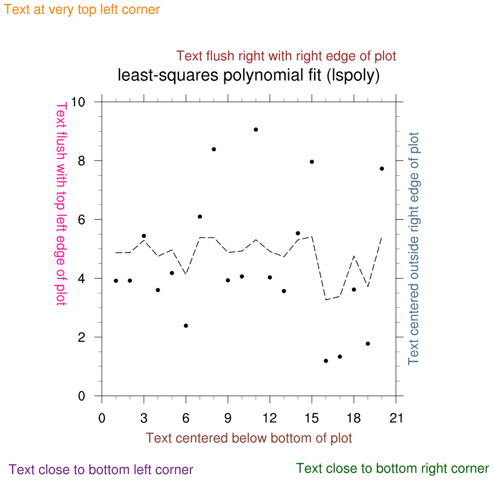
 text_20.ncl
: This example shows how
to use the
drawNDCGrid procedure
to help you select locations for placing text outside the plot.
The first image is the plot with the NDC grid. The second image is
the plot with text strings added.
Once the XY plot is created, you can use
setvalues
to retrieve the viewport area of the plot, and
NhlGetBB to retrieve the bounding box that encloses all the
plot elements. This allows you to calculate the location of various text strings
relative to the plot's size and location.


