NCL Graphics: Toulouse Models

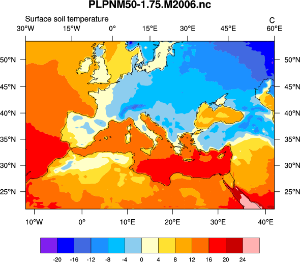ALADIN_tsur_5.ncl: This script plots the surface soil temperature ("tsur") from the ALADIN model on a lambert conformal map. The data were provided by Pierre Nabat of Météo-France.

The lambert conformal projection information was written to the file via the "Lambert_Conformal" variable, so we were able to use this to set the special lambert parallel and merdian resources.

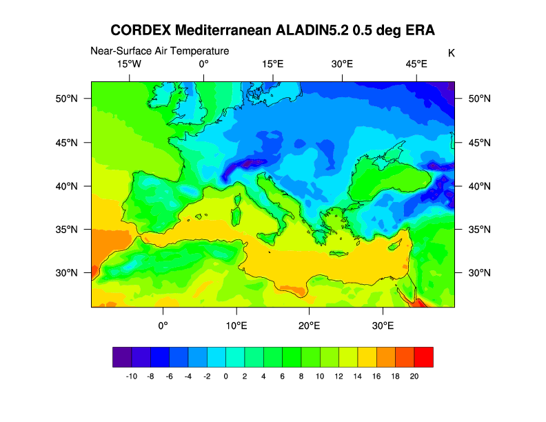ALADIN_tas_5.ncl: This script is similar to the previous "ALADIN_tsur_5.ncl" script. The data file was provided by Samuel Somot of Météo-France.

It plots the near-surface air temperature ("tas") from an ALADIN file, putting it on a lambert conformal projection.

To create an animated GIF of this variable which has 384 time steps, run ALADIN_tas_anim.ncl. The cd_calendar function is used to create a time stamp as the main title.

To create the GIF file, you must have the free convert tool from ImageMagick installed. A file called ALADIN_tas_anim.gif will be created, which you can open with your web browser to see the animation. In the script, every 10th timestep is plotted. This was to keep the GIF file small. To plot every time step, simply remove the ",10" from the do loop.

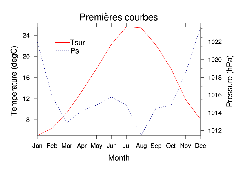ALADIN_tsur_mslp.ncl: This script creates a time series plot of averaged temperature and pressure on the same page, using different labels on the right and left Y axis. It shows how to create text labels that contain French accented characters, like è.

It was created by Pierre Nabat during the NCL Workshop at CERFACS, October 4-5, 2012.

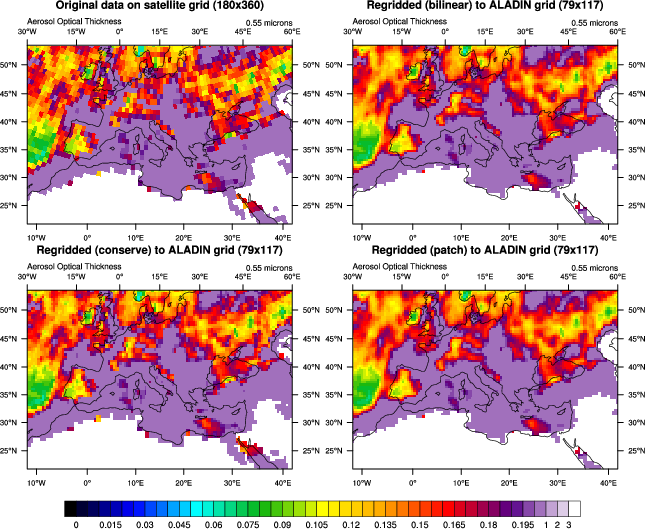Sat_to_ALADIN_regrid.ncl: This script shows how to regrid data on a satellite grid to an ALADIN grid using three different ESMF regridding methods (bilinear, conserve, patch).

The datasets were provided bymodel on a lambert conformal map. The data were provided by Pierre Nabat of Météo-France.

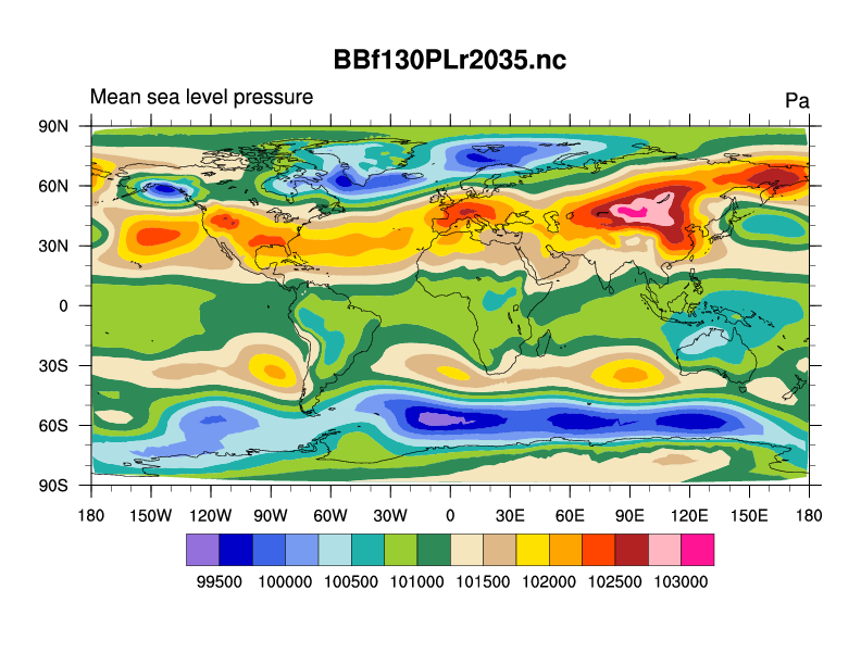
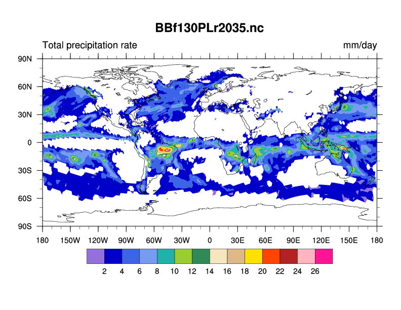ARPEGE_BB.ncl: This script shows how to plot data from an ARPEGE model. The NetCDF file used for these plots is "BBf130PLr2035.nc", provided by Silvana Buarque of Météo-France.

You can modify this script to change which variables you want to plot by changing the "varc" line.

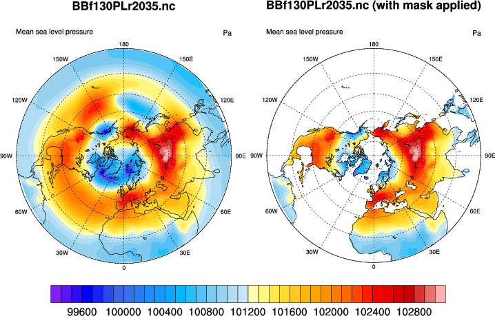ARPEGE_BB_mask.ncl: This script reads "psl" from the same dataset as the previous example, and applies an inverted sea-land mask (from a separate NetCDF file) to it using the where function.

Contours of the original data and the masked data are "paneled" on the same page using gsn_panel.

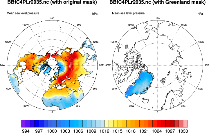ARPEGE_BB_Greenland_mask.ncl: This script was created during the workshop (and improved after the workshop) based on questions from Silvana. She wanted to mask her data roughly over the area of Greenland. A Greenland shapefile was downloaded from www.gadm.org/country and used to create a new mask.

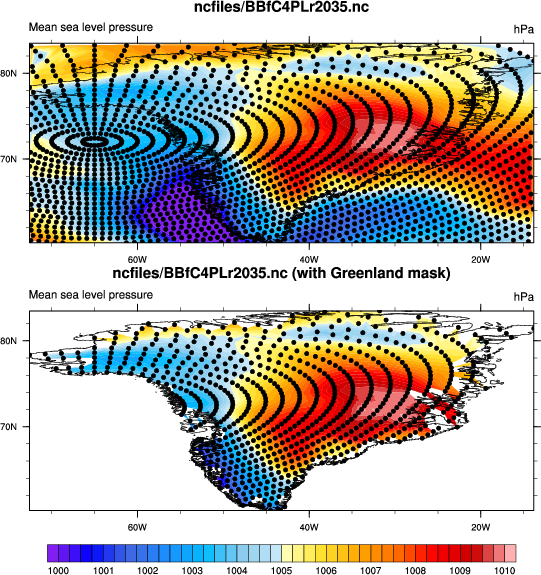ARPEGE_psl_with_GRL_mask_and_grid.ncl: This example uses the "greenland_mask.nc" mask file created in the previous "ARPEGE_BB_Greenland_mask.ncl" script, and draws a plot of "psl" and "masked psl" with the lat/lon grid locations drawn as filled dots.

If you are using NCL V6.0.0 or earlier, then you need to download this gsn_coordinates.ncl script.

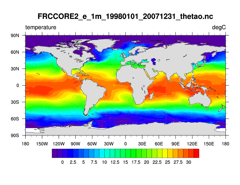IPSL_thetao.ncl: This script plots "thetao" from an IPSL climate model dataset, provided by Sophie Valcke of CERFACS.

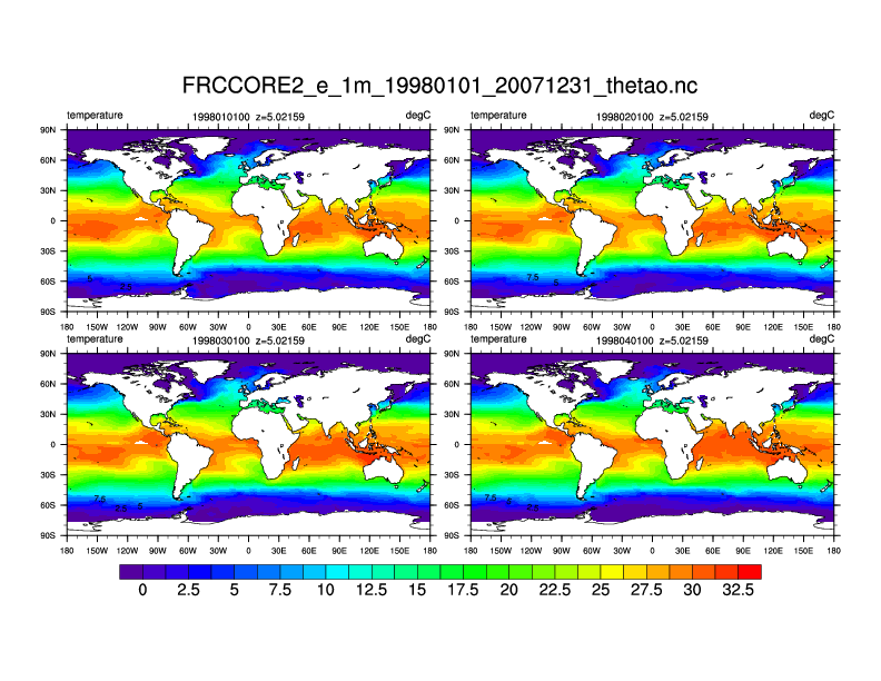IPSL_thetao_panel.ncl: This script is similar to the previous one, except it creates four plots of thetao using a different timestep, and then panels them with gsn_panel.

To create an animated GIF of this variable across all 120 timesteps, run IPSL_thetao_anim.ncl. You must have the free convert tool from ImageMagick installed to create the GIF file. The cd_calendar function is used to create a time stamp as the main title.

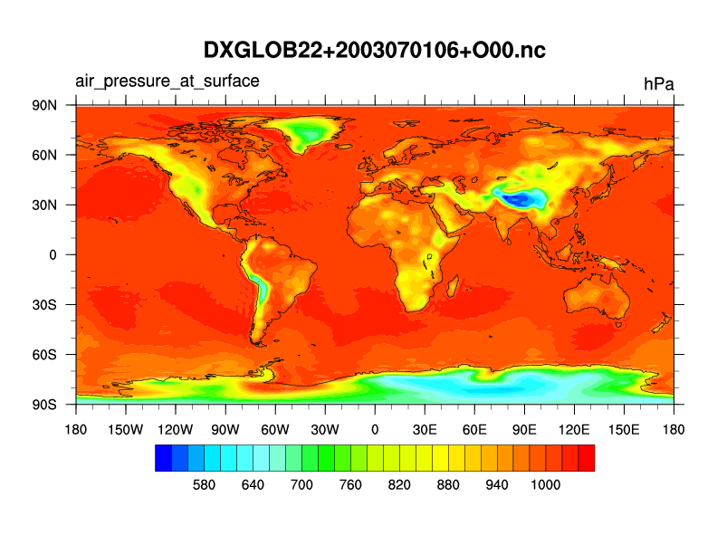MOCAGE_DX_apas.ncl: This script plots "apas" (pressure) from a MOCAGE model dataset, provided by Andrea Piacentini of CERFACS.

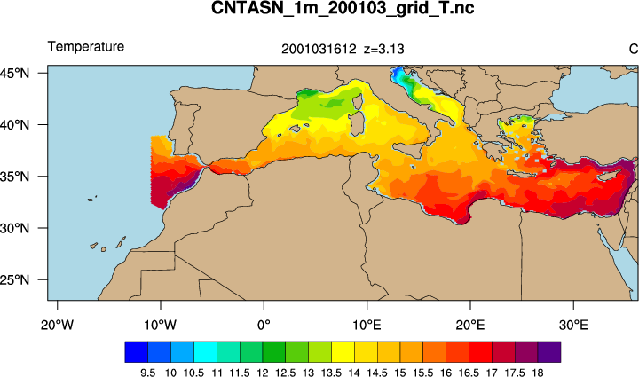NEMO_CNTASN_temper.ncl: This script shows how to plot "votemper" (temperature) from a NEMO file provided by Clotilde Dubois of Météo-France.

Optionally, you can set USE_SHAPEFILE to True to draw country outlines from a shapefile instead of using NCL map outlines. To use the shapefile outlines, you must download the "country bounaries" shapefile data from http://www.diva-gis.org/Data/.

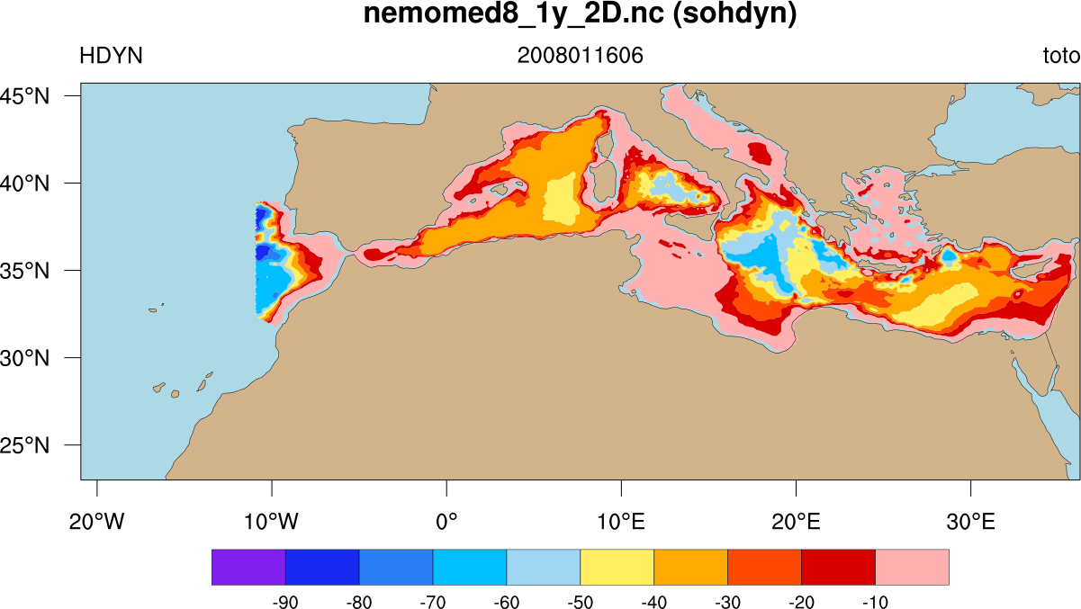
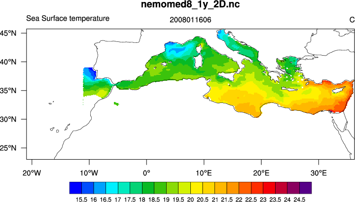NEMO_sst.ncl: This script shows how to plot "sosstsst" (sea surface temperature) from a NEMO file provided by Florence Sevault of Météo-France.

The missing values for this variable had to be "fixed" because they were not exactly equal to the sst@_FillValue value. This was done by using the where function to set all values greater-than-or-equal to sst@_FillValue to sst@_FillValue.

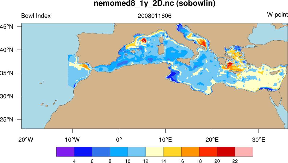
NEMO_plot_all.ncl: This script shows how to plot the first timestep of every three-dimensional numeric variable on a NEMO data file. The purpose of this is to get a quick visual look at the data on the file.

The getfilevarnames function is used to read all the variable names off the file. The isnumeric and dimsizes functions are then used to check if this variable is numeric and how many dimensions it has.

Each variable is plotted to its own PNG file.

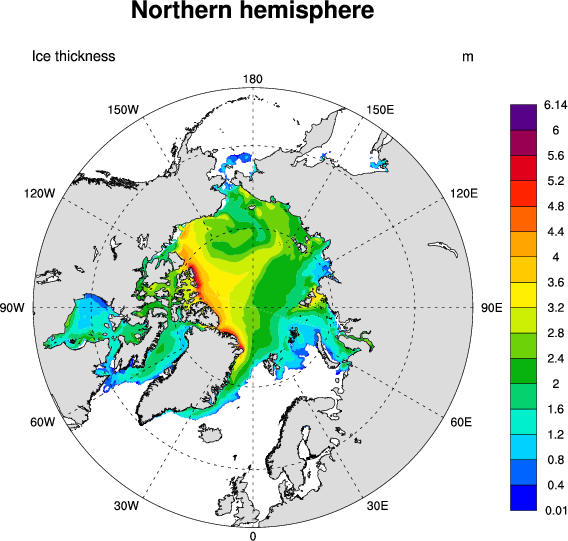
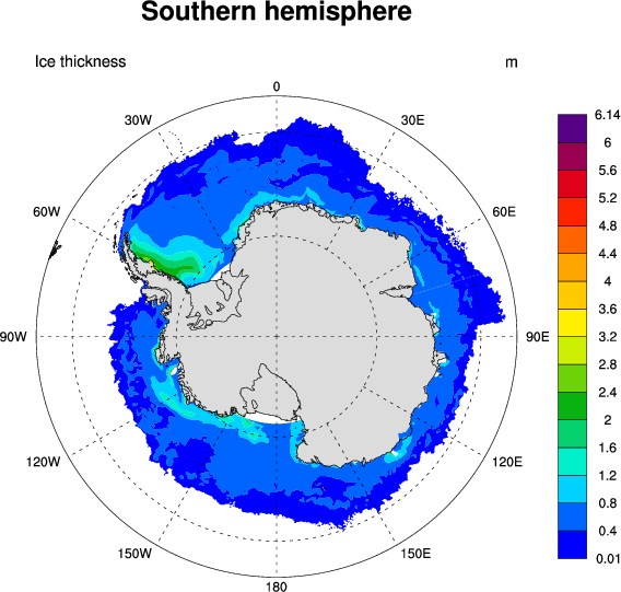ORCA025_icemod.ncl: This script shows how to plot ice thickness from an ORCA 0.25 degree grid file provided by Romain Bourdalle-Badie of Mercator Ocean. The variable is dimensioned 1021 x 1442.

The "iicethic" variable is of type "short" on the file, with a "scale_factor" that needs to be applied, so short2flt is used to do the conversion.

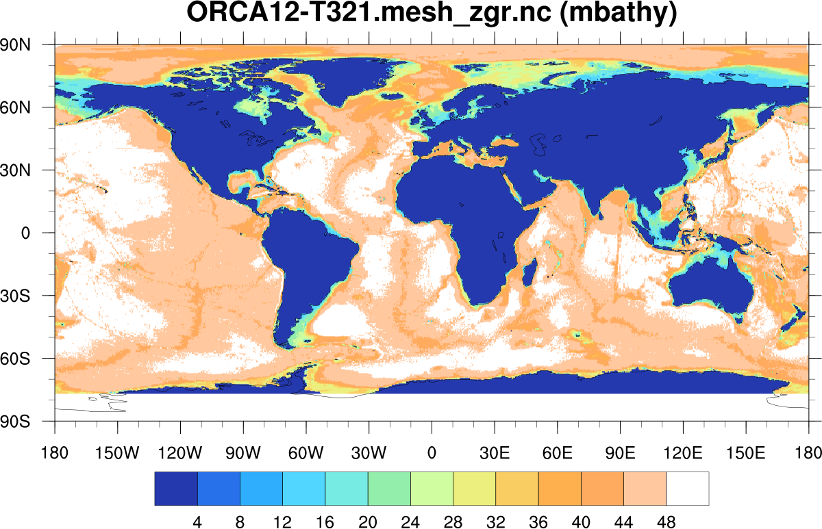ORCA12_zgr_mbathy.ncl: This script shows how to plot bathymetry from an ORCA12 grid file provided by Romain Bourdalle-Badie of Mercator Ocean. The variable is dimensioned 3059 x 4322, so it takes awhile longer to plot.

For faster plotting, it's important to set:

res@cnFillMode = "RasterFill"
res@trGridType = "TriangularMesh"

When NCL V6.1.0 is released, you can try an experimental fill mode of "MeshFill" for even faster plotting.

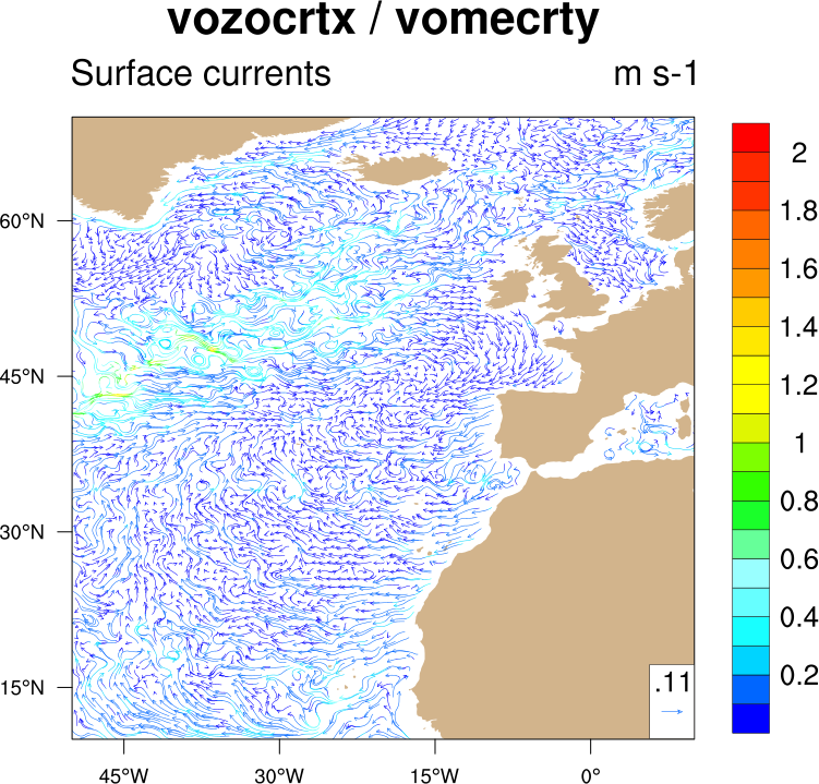ORCA12_gridUV_vel.ncl: This example shows how to created a curly vector plot that is colored based on magnitude. This is a large grid (3059 x 4322), so only every 10th data value is plotted.

For an example of plotting the full grid, see the "ORCA12_gridUV_vel_3.ncl" script at http://www.ncl.ucar.edu/Training/Workshops/CERFACS/Scripts/ORCA/.

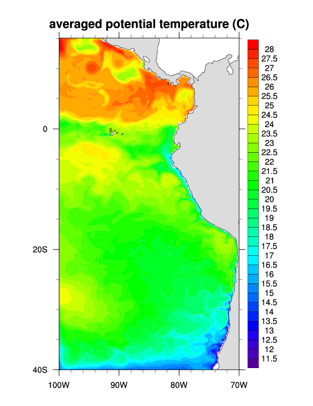ROMS_avgtemp.ncl: This script shows how to plot average potential temperature from a ROMS file provided by Séréna Thevenin-Illig of LEGOS. The lat/lon coordinates are read off a separate file.

All temperature values equal to 0.0 are set to a missing value so they don't get plotted. This effectively masks out the land values.

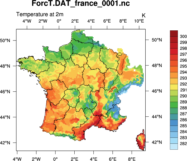
SAFRAN_temperature.ncl: This script shows how to plot temperature from a SAFRAN file provided by Clotilde Dubois of Météo-France.

If USE_SHAPEFILE is set to True, then you must download the France shapefile data from www.gadm.org/country.

This script uses the "WhiteBlueGreenYellowRed" color table, which has several very light shades of white and blue at the beginning that we may not want. To remove these, you can read in the color table with read_colormap_file, and then subset as necessary when setting the cnFillPalette resource.

SAFRAN_temperature_anim.ncl: This script is similar to the previous one, except it creates an animated GIF image from every 24 timesteps (they are hourly). The cd_string function is used to create a time stamp as the main title.

After about time index 2991, the time values suddenly go to 0, so we have cull these values out by using ind to get only the time values that are > 0.

You must have the free convert tool from ImageMagick installed to create the GIF file.

Click on the thumbnail to see the animation.

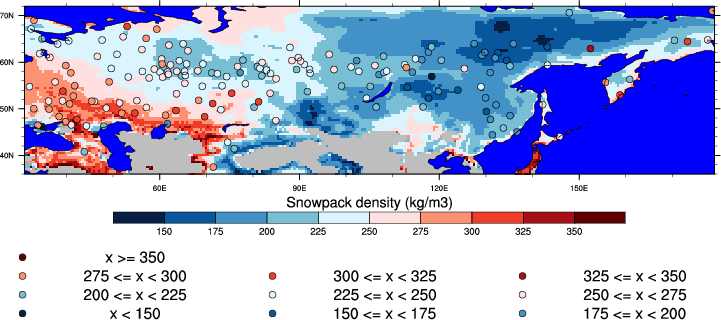snow_density_map.ncl: This script was written by Eric Brun and Stéphane Senesi of Météo-France during the NCL workshop. It compares snowpack density from observations read off an ASCII file with Crocus snow model output read off a NetCDF file.