NCL Home>
Application examples>
Data sets ||
Data files for some examples

 gfed_2.ncl:
Open a GFED hdf5 file; read and plot specified variables from different groups.
This example uses the where function and the variable basis_regions
contained within the ancill group to mask areas.
The stat_dispersion function is used to examine the
variable's distribution.
gfed_2.ncl:
Open a GFED hdf5 file; read and plot specified variables from different groups.
This example uses the where function and the variable basis_regions
contained within the ancill group to mask areas.
The stat_dispersion function is used to examine the
variable's distribution.
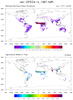
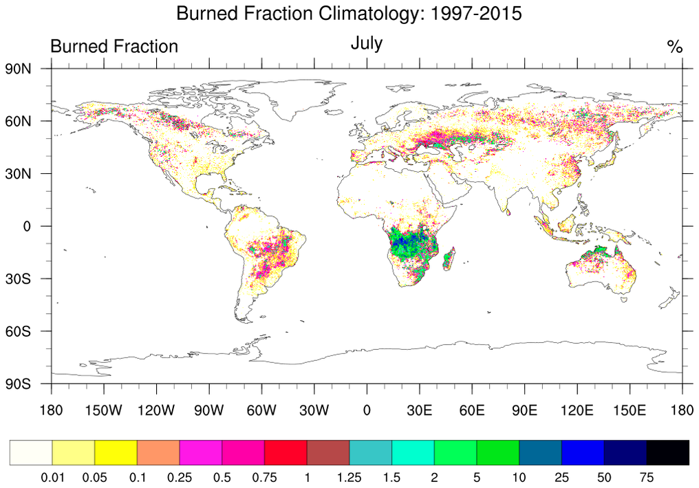
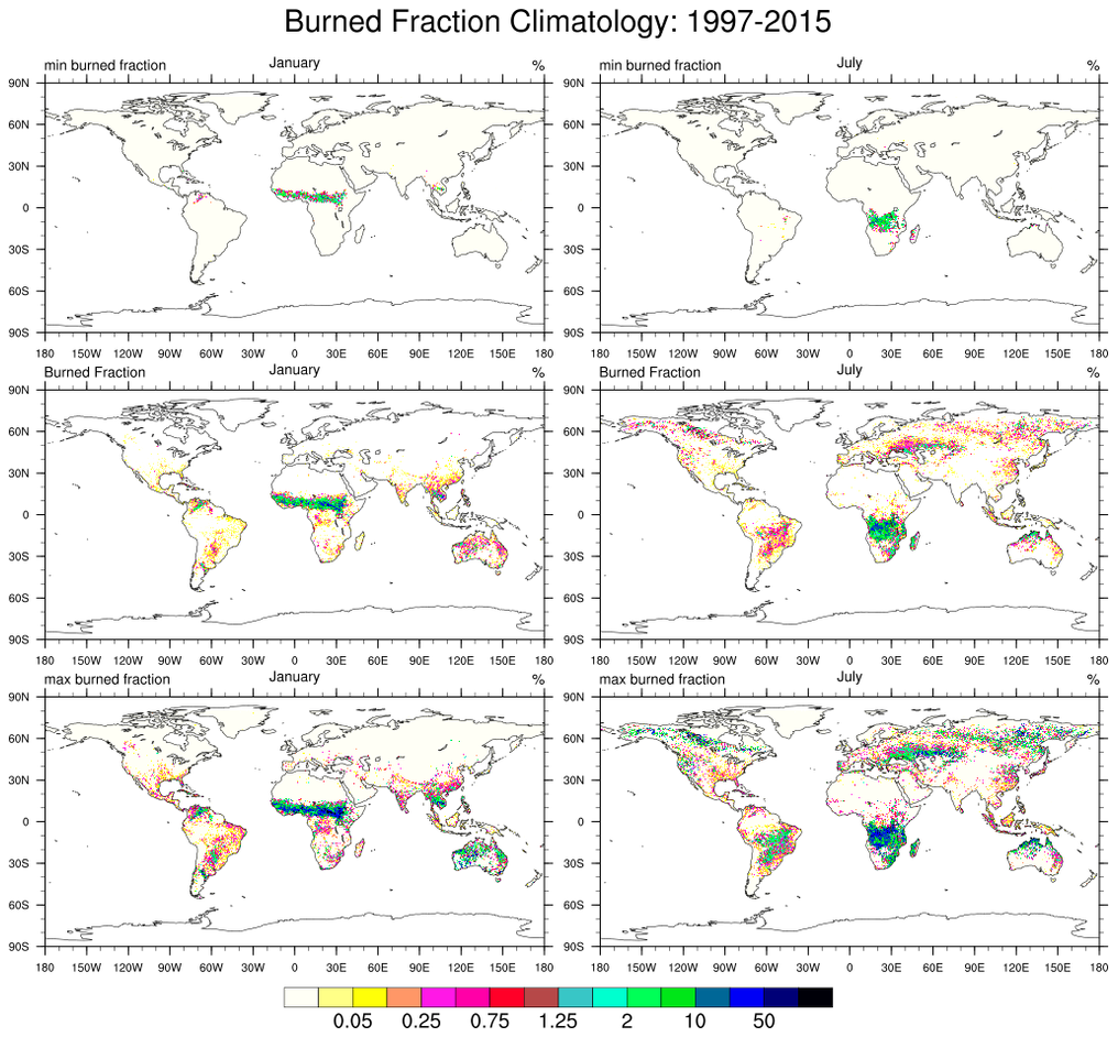
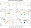 gfed_5.ncl:
Open a single variable netCDF-4 file containing data for all years (See Example 4).
Compute and plot: (a) monthly climatology and (b) the minimum and maximum values
over all the available years. The left plot shows the climatological JULY "burned fraction (%)."
The right figures shows the climatological minimum (top), mean (middle) and maximum (bottom)
for January and July.
gfed_5.ncl:
Open a single variable netCDF-4 file containing data for all years (See Example 4).
Compute and plot: (a) monthly climatology and (b) the minimum and maximum values
over all the available years. The left plot shows the climatological JULY "burned fraction (%)."
The right figures shows the climatological minimum (top), mean (middle) and maximum (bottom)
for January and July.
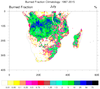

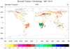
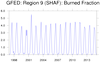 gfed_6.ncl:
Open a single variable netCDF-4 file containing data for all years.
Specify a region; use 'basis-region' to extract only desired variables; extract and plot. Compute and plot:
(a) monthly climatology and (b) the minimum and maximum values over all the available years.
Also calculate and plot the areal average (wgt_areaave2 using
the 'GRID_CELL_AREA' variable for each time step).
gfed_6.ncl:
Open a single variable netCDF-4 file containing data for all years.
Specify a region; use 'basis-region' to extract only desired variables; extract and plot. Compute and plot:
(a) monthly climatology and (b) the minimum and maximum values over all the available years.
Also calculate and plot the areal average (wgt_areaave2 using
the 'GRID_CELL_AREA' variable for each time step).
Example pages containing:
tips |
resources |
functions/procedures
NCL: GFED: Global Fire Emissions Database
The Global Fire Emissions Database (GFED) provides
"combined satellite information on fire activity and vegetation productivity to estimate
gridded monthly burned area and fire emissions, as well as scalars that can be used to
calculate higher temporal resolution emissions."
The GFED files are archived in HDF5 format. NCL's
ncl_filedump
(here)
or Unidata's ncdump -h
(here)
may be used to examine a GFED's HDF5 file's contents.
            ncl_filedump GFED4.1s_1997.hdf5 | less
            ncdump -h GFED4.1s_1997.hdf5 | less
The information on each output files is the same. However, there are some differences in
the presentation. For NCL applications, it is recommended that users use the
ncl_filedump as a reference because that is how NCL 'sees' the file.
The hdf5 file structure uses multiple embedded groups. The group names are: ancill, biosphere, burned_area and emissions. The latter three groups are further enclosed within monthly groups named 01, 02,...,12. Each monthly group contains several variables. Lastly, the emissions group has a sub-group named partitioning which contains category emissions.
NCL can readily access the groups and variables on the hdf5 files (See Examples 1-3.) However, the multiple embedded groups are cumbersome. To facilitate CESM related objectives, NCL scripts were used to create Climate and Forecast (CF) conforming netCDF files with two different variable arrangements. (See Examples 3 and 4.)
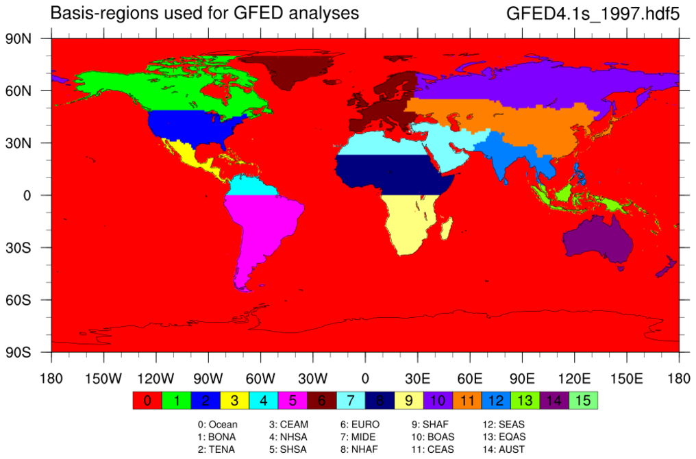
The source GFED grids are rectilinear with 0.25 degree resolution (720x1440) with North-to-South (89.875N to 89.875S) and longitudes spanning (-179.875 to 179.875) in longitude. Further, a regional mask is provided that readily allows regional data to be extracted. Specifically:
   basis_regions(720,1440) ;
           string basis_regions:long_name = "Basis-regions used for GFED analyses" ;

           string basis_regions:class_0 = "Ocean" ;
           string basis_regions:class_1 = "BONA (Boreal North America)" ;
           string basis_regions:class_2 = "TENA (Temperate North America" ;
           string basis_regions:class_3 = "CEAM (Central America)" ;
           string basis_regions:class_4 = "NHSA (Northern Hemisphere South America)" ;
           string basis_regions:class_5 = "SHSA (Southern Hemisphere South America)" ;
           string basis_regions:class_6 = "EURO (Europe)" ;
           string basis_regions:class_7 = "MIDE (Middle East)" ;
           string basis_regions:class_8 = "NHAF (Northern Hemisphere Africa)" ;
           string basis_regions:class_9 = "SHAF (Southern Hemisphere Africa)" ;
           string basis_regions:class_10 = "BOAS (Boreal Asia)" ;
           string basis_regions:class_11 = "CEAS (Central Asia)" ;
           string basis_regions:class_12 = "SEAS (Southeast Asia)" ;
           string basis_regions:class_13 = "EQAS (Equatorial Asia)" ;
           string basis_regions:class_14 = "AUST (Australia and New Zealand)" ;
Please also see the Climate Analysis Section's Climate Data Guide
for further information on the monthly products. Search for GFED.
 gfed_2.ncl:
Open a GFED hdf5 file; read and plot specified variables from different groups.
This example uses the where function and the variable basis_regions
contained within the ancill group to mask areas.
The stat_dispersion function is used to examine the
variable's distribution.
gfed_2.ncl:
Open a GFED hdf5 file; read and plot specified variables from different groups.
This example uses the where function and the variable basis_regions
contained within the ancill group to mask areas.
The stat_dispersion function is used to examine the
variable's distribution.
gfed_3.ncl:
Convert all yearly (12 months) GFED HDF5 files [GFED4.1s_YYYY.hdf5]
to netCDF-4 to facilitate use for CESM post-processing.
Specifically, a source file named 'GFED4.1s_1997.hdf5'
will yield a corresponding netCDF-4 file named 'GFED4.1s_1997.nc'.
Further, the grids will be ordered South-to-North and (-87.875 to 87.875) the longitudes will span 0.125-to-359.875 to facilitate CESM post-processing. The created file(s) will contain classic coordinate variables [(time,lat,lon)] with temporal information. A sample ncdump -h of the newly created netCDF-4 file for 1997 is (here)
gfed_3.beta_monthly.ncl: Extract the monthly variables only from a GFED file containing monthly and daily values. Specifically, a source file named 'GFED4.1s_2017_beta.hdf5' will produce a file named: 'GFED4.1s_2017.nc'. The variables will be: (time,lat,lon)=>(12,360,720).
gfed_3.beta_daily.ncl: Extract the daily variables only from a GFED file containing monthly and daily values. Specifically, a source file named 'GFED4.1s_2017_beta.hdf5' will produce a file named: 'GFED4.1s_2017.daily_fraction.nc'. The variable will be: (time,lat,lon)=>(365,360,720). A leap year would be: (366,360,720).
gfed_4.ncl:
Use NCL as a scripting language to invoke the
netCDF operator (ncrcat)
to create single-variable netCDF-4 files. A sample ncdump -h
of a GFED single-variable netCDF file is
here.
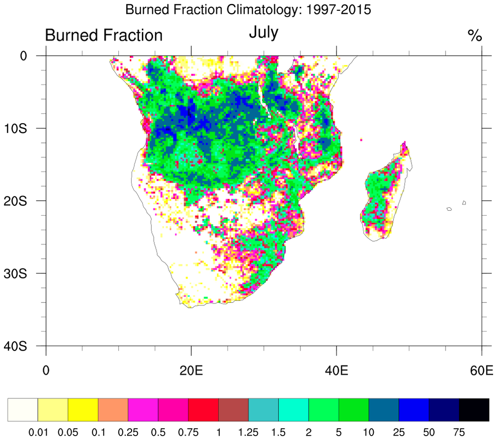
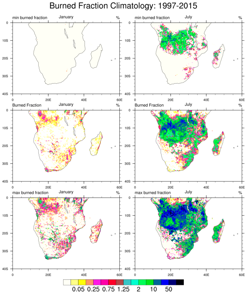
 gfed_5.ncl:
Open a single variable netCDF-4 file containing data for all years (See Example 4).
Compute and plot: (a) monthly climatology and (b) the minimum and maximum values
over all the available years. The left plot shows the climatological JULY "burned fraction (%)."
The right figures shows the climatological minimum (top), mean (middle) and maximum (bottom)
for January and July.
gfed_5.ncl:
Open a single variable netCDF-4 file containing data for all years (See Example 4).
Compute and plot: (a) monthly climatology and (b) the minimum and maximum values
over all the available years. The left plot shows the climatological JULY "burned fraction (%)."
The right figures shows the climatological minimum (top), mean (middle) and maximum (bottom)
for January and July.
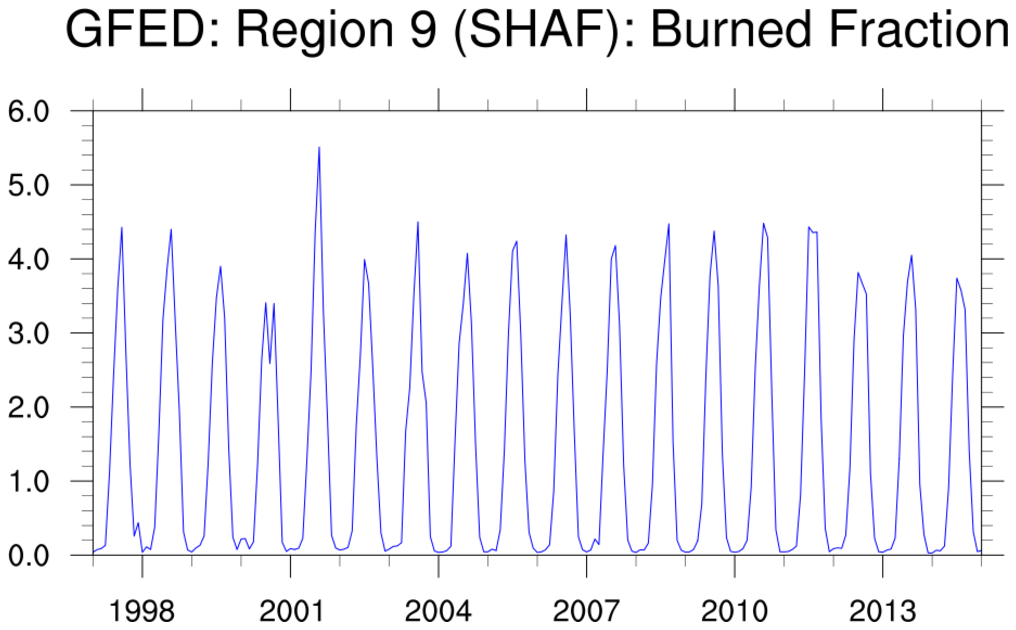 gfed_6.ncl:
Open a single variable netCDF-4 file containing data for all years.
Specify a region; use 'basis-region' to extract only desired variables; extract and plot. Compute and plot:
(a) monthly climatology and (b) the minimum and maximum values over all the available years.
Also calculate and plot the areal average (wgt_areaave2 using
the 'GRID_CELL_AREA' variable for each time step).
gfed_6.ncl:
Open a single variable netCDF-4 file containing data for all years.
Specify a region; use 'basis-region' to extract only desired variables; extract and plot. Compute and plot:
(a) monthly climatology and (b) the minimum and maximum values over all the available years.
Also calculate and plot the areal average (wgt_areaave2 using
the 'GRID_CELL_AREA' variable for each time step).