NCL Home>
Application examples>
Data Analysis ||
Data files for some examples
 grid_fill_1.ncl:
For demonstration purposes, create a grid using generate_2d_array;
then use array syntax to set regions to missing values [_FillValue].
Use poisson_grid_fill to fill the missing regions.
The top plot is the original grid; the middle plot shows the regions
which were manually set to _FillValue; the bottom plot show the
plot after poisson_grid_fill was used.
grid_fill_1.ncl:
For demonstration purposes, create a grid using generate_2d_array;
then use array syntax to set regions to missing values [_FillValue].
Use poisson_grid_fill to fill the missing regions.
The top plot is the original grid; the middle plot shows the regions
which were manually set to _FillValue; the bottom plot show the
plot after poisson_grid_fill was used.
 grid_fill_2.ncl:
Read SST data which contains missing values (_FillValue) over land.
Use poisson_grid_fill to fill the missing regions.
The left plot show the global reconstruction; the right plot shows
the result when operating over a limited region. Note that
the values over South America were extrapolted.
grid_fill_2.ncl:
Read SST data which contains missing values (_FillValue) over land.
Use poisson_grid_fill to fill the missing regions.
The left plot show the global reconstruction; the right plot shows
the result when operating over a limited region. Note that
the values over South America were extrapolted.

 grid_fill_3.ncl:
Read hybrid model level data; use vinth2p or
vinth2p_ecmwf to interpolate the data
to user specified constant pressure levels. Data below
the surface pressure [PS] are not available. Hence,
extrapolation or grid filling (poisson_grid_fill)
must be used.
grid_fill_3.ncl:
Read hybrid model level data; use vinth2p or
vinth2p_ecmwf to interpolate the data
to user specified constant pressure levels. Data below
the surface pressure [PS] are not available. Hence,
extrapolation or grid filling (poisson_grid_fill)
must be used.
 grid_fill_4.ncl:
This is similar to example 3. Here the focus was in a region which
included the Himalaya rather than the globe. It more clearly
illustrates the strengths/weaknesses
of vinth2p_ecmwf and
poisson_grid_fill.
grid_fill_4.ncl:
This is similar to example 3. Here the focus was in a region which
included the Himalaya rather than the globe. It more clearly
illustrates the strengths/weaknesses
of vinth2p_ecmwf and
poisson_grid_fill.
 grid_fill_5.ncl:
SMOPS (Soil Moisture Operational Products System) estimates for a day are read.
There are 'swath gaps' over land which contain _FillValue. These are colored as yellow
in the figures. NCL's poisson_grid_fill is used to fill
these gaps. It also fills all grid points with _FillValue. NCL's
landsea_mask is used to mask ocean, inland water and
ice regions.
grid_fill_5.ncl:
SMOPS (Soil Moisture Operational Products System) estimates for a day are read.
There are 'swath gaps' over land which contain _FillValue. These are colored as yellow
in the figures. NCL's poisson_grid_fill is used to fill
these gaps. It also fills all grid points with _FillValue. NCL's
landsea_mask is used to mask ocean, inland water and
ice regions.
 MOPITT_MOP03M_3.ncl:
Read a variable and interpolate to a much coarser 46x72 grid using
linint2_Wrap and
area_hi2lores_Wrap.
Missing areas are present. Then use poisson_grid_fill
to fill in the missing values and repeat the interpolations.
MOPITT_MOP03M_3.ncl:
Read a variable and interpolate to a much coarser 46x72 grid using
linint2_Wrap and
area_hi2lores_Wrap.
Missing areas are present. Then use poisson_grid_fill
to fill in the missing values and repeat the interpolations.
Example pages containing: tips | resources | functions/procedures
NCL: Grid Filling
Sometimes, it is desirable to 'fill' regions containing
missing values [_FillValue] with interpolated values while
leaving the original values unchanged.
poisson_grid_fill performs this task.
Input values are unchanged and act a boundary conditions (constraints).
Generally, in regions bounded by valid data, this function does a
'pretty good job'. This function will extrapolate beyond data boundaries
and, as always, extrapolated values should be used with caution.
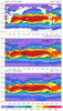
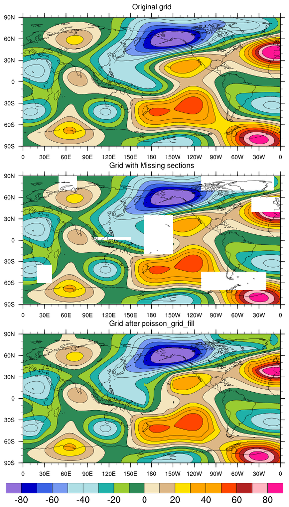 grid_fill_1.ncl:
For demonstration purposes, create a grid using generate_2d_array;
then use array syntax to set regions to missing values [_FillValue].
Use poisson_grid_fill to fill the missing regions.
The top plot is the original grid; the middle plot shows the regions
which were manually set to _FillValue; the bottom plot show the
plot after poisson_grid_fill was used.
grid_fill_1.ncl:
For demonstration purposes, create a grid using generate_2d_array;
then use array syntax to set regions to missing values [_FillValue].
Use poisson_grid_fill to fill the missing regions.
The top plot is the original grid; the middle plot shows the regions
which were manually set to _FillValue; the bottom plot show the
plot after poisson_grid_fill was used.

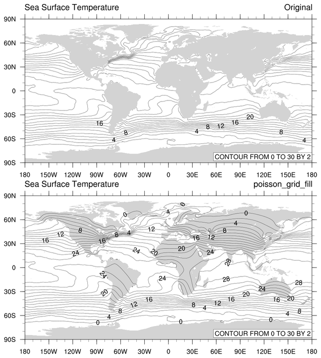
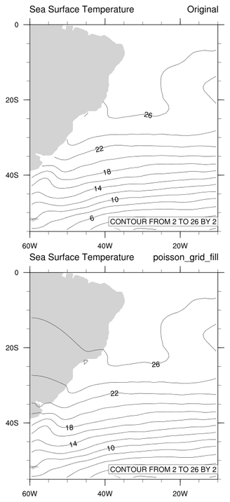 grid_fill_2.ncl:
Read SST data which contains missing values (_FillValue) over land.
Use poisson_grid_fill to fill the missing regions.
The left plot show the global reconstruction; the right plot shows
the result when operating over a limited region. Note that
the values over South America were extrapolted.
grid_fill_2.ncl:
Read SST data which contains missing values (_FillValue) over land.
Use poisson_grid_fill to fill the missing regions.
The left plot show the global reconstruction; the right plot shows
the result when operating over a limited region. Note that
the values over South America were extrapolted.
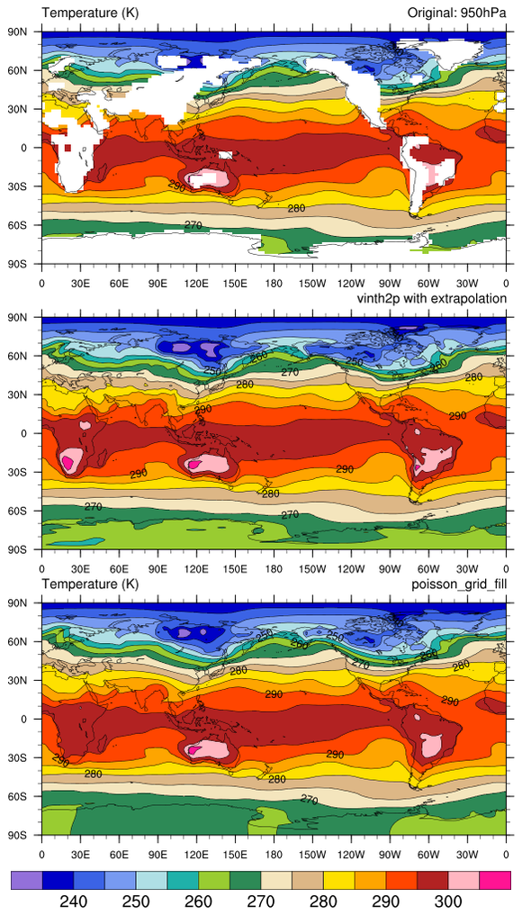
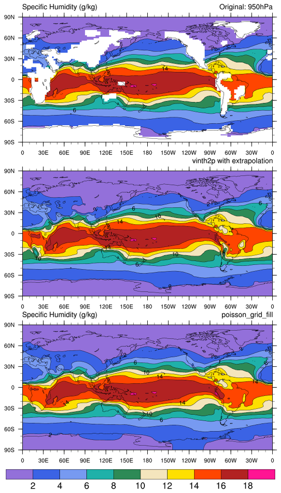
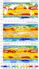
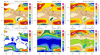
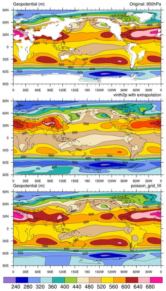 grid_fill_3.ncl:
Read hybrid model level data; use vinth2p or
vinth2p_ecmwf to interpolate the data
to user specified constant pressure levels. Data below
the surface pressure [PS] are not available. Hence,
extrapolation or grid filling (poisson_grid_fill)
must be used.
grid_fill_3.ncl:
Read hybrid model level data; use vinth2p or
vinth2p_ecmwf to interpolate the data
to user specified constant pressure levels. Data below
the surface pressure [PS] are not available. Hence,
extrapolation or grid filling (poisson_grid_fill)
must be used.
For demonstration purposes the 950 hPa level was chosen. In each figure the top plot shows the original grid. The clear areas represent regions where 950hPa was below the corresponding surface pressure. The middle plots show the result after using vinth2p_ecmwf to interpolate temperature, specific humidity and geopotential height. The bottom plot shows the result after using poisson_grid_fill.
If the clear areas is bounded by valid grid points, the poisson_grid_fill produces reasonable patterns. The area where values look unreasonable are the grid points over the Antarctic. This is because to points are not bounded. The vinth2p_ecmwf has problems when it is used to extrapolate at levels well below the surface pressure level.
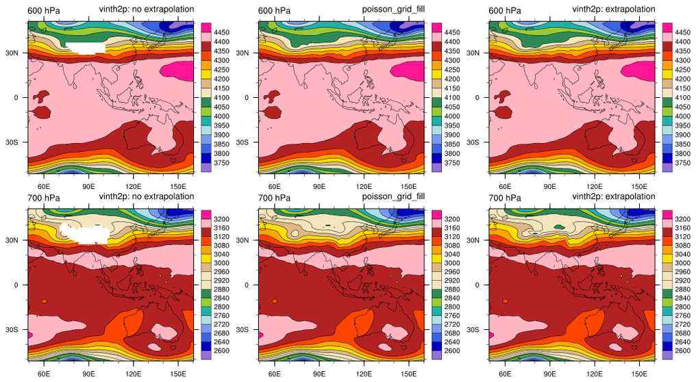
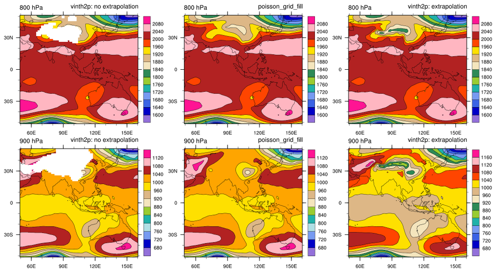
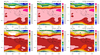
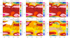
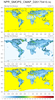
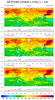
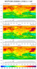
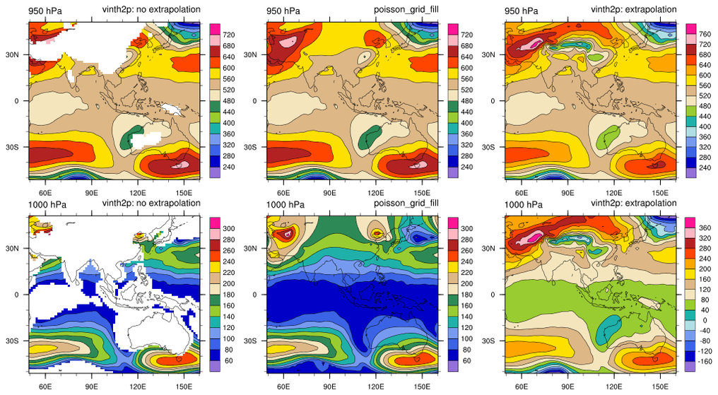 grid_fill_4.ncl:
This is similar to example 3. Here the focus was in a region which
included the Himalaya rather than the globe. It more clearly
illustrates the strengths/weaknesses
of vinth2p_ecmwf and
poisson_grid_fill.
grid_fill_4.ncl:
This is similar to example 3. Here the focus was in a region which
included the Himalaya rather than the globe. It more clearly
illustrates the strengths/weaknesses
of vinth2p_ecmwf and
poisson_grid_fill.
The Z3 variable is interpolated to constant pressure levels. The constant pressure levels include 600, 700, 800, 900, 950, 1000. Each of the 3 images contains two horizontal rows. The leftmost plot contains the 600 & 700hPa levels; the middle image the 800 & 900hPa levels; the rightmost imnage the 950 & 1000 hPa levels. The left figure of each plot shows the interpolated Z3 with no extrapolation. Non-colored areas indicate regions (grid points) that are below the surface pressure. The middle plots show the level after interpolation by poisson_grid_fill. The rightmost plots show the result of applying vinth2p_ecmwf.
Note that the poisson_grid_fill (middle) plots generally look "reasonable" as long as there are boundary values. Clearly the 1000 hPa level at the northern boundary look unusual. At the lower levels the vinth2p_ecmwf are on a different scale.
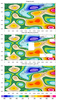
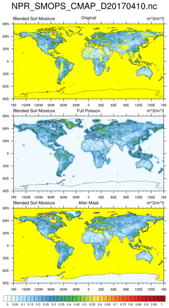 grid_fill_5.ncl:
SMOPS (Soil Moisture Operational Products System) estimates for a day are read.
There are 'swath gaps' over land which contain _FillValue. These are colored as yellow
in the figures. NCL's poisson_grid_fill is used to fill
these gaps. It also fills all grid points with _FillValue. NCL's
landsea_mask is used to mask ocean, inland water and
ice regions.
grid_fill_5.ncl:
SMOPS (Soil Moisture Operational Products System) estimates for a day are read.
There are 'swath gaps' over land which contain _FillValue. These are colored as yellow
in the figures. NCL's poisson_grid_fill is used to fill
these gaps. It also fills all grid points with _FillValue. NCL's
landsea_mask is used to mask ocean, inland water and
ice regions.
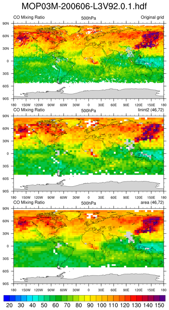
 MOPITT_MOP03M_3.ncl:
Read a variable and interpolate to a much coarser 46x72 grid using
linint2_Wrap and
area_hi2lores_Wrap.
Missing areas are present. Then use poisson_grid_fill
to fill in the missing values and repeat the interpolations.
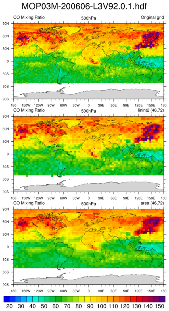
MOPITT_MOP03M_3.ncl:
Read a variable and interpolate to a much coarser 46x72 grid using
linint2_Wrap and
area_hi2lores_Wrap.
Missing areas are present. Then use poisson_grid_fill
to fill in the missing values and repeat the interpolations.