NCL: Spectral Analysis and Complex Demodulation

Spectral Analysis

Spectral analysis of time series is the process of partitioning the temporal variance information into frequency variance information. The latter is called the spectrum. The spectrum breaks the sample variance of time series into discret components, each of which is associated with a particular frequency.

A nice simple example of the concept and process is provided at Introduction to Spectral Analysis (D. Percival, U. Washington).

The NCL functions specx_anal and specxy_anal perform the temporal-to-frequency transformation via the Fast Fourier Transform (FFT). The FFT implicitly assume the time series are 'cyclic'. Generally, this is not true. Hence, the source time series must be pre-treated (aka, "pre-whitening"). In most applications, this means the data must be tapered in the time or frequency domains. NCL's functions perform the tapering in the time domain. Further, removing any linear trend in the source data is recommended. The trend removal is performed first, then the trend-removed data are tapered. This combination minimizes "ringing" and "leakage".

The FFT performed on the pre-whitened series create periodogram estimates. Nominally, each periodogram estimate has 2 degrees of freedom for each frequency band. ("Nominally" because the source data has been pre-whitened which slightly reduces the degrees of freedom..) To provide some level of statistical reliability, the periodogram estimates must be smoothed. For example, a 5-point smoother would nominally result in 10 degrees of freedom (5*2). The side effect of the smoothing process is that the effective band-width is wider (think, 5*periodogram-band-width). A nice description is at: Spectral Analysis: Smoothed Periodogram Method (DMeko, U. Arizona).

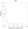spec_1.ncl: Reads in a time series from a netCDF file, calculates the spectrum and plots the results.

specx_anal: Calculates the spectra of a time series with options on smoothing, demeaning, detrending, and tapering.

dimsizes: calculates the dimension sizes of any array.

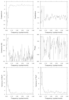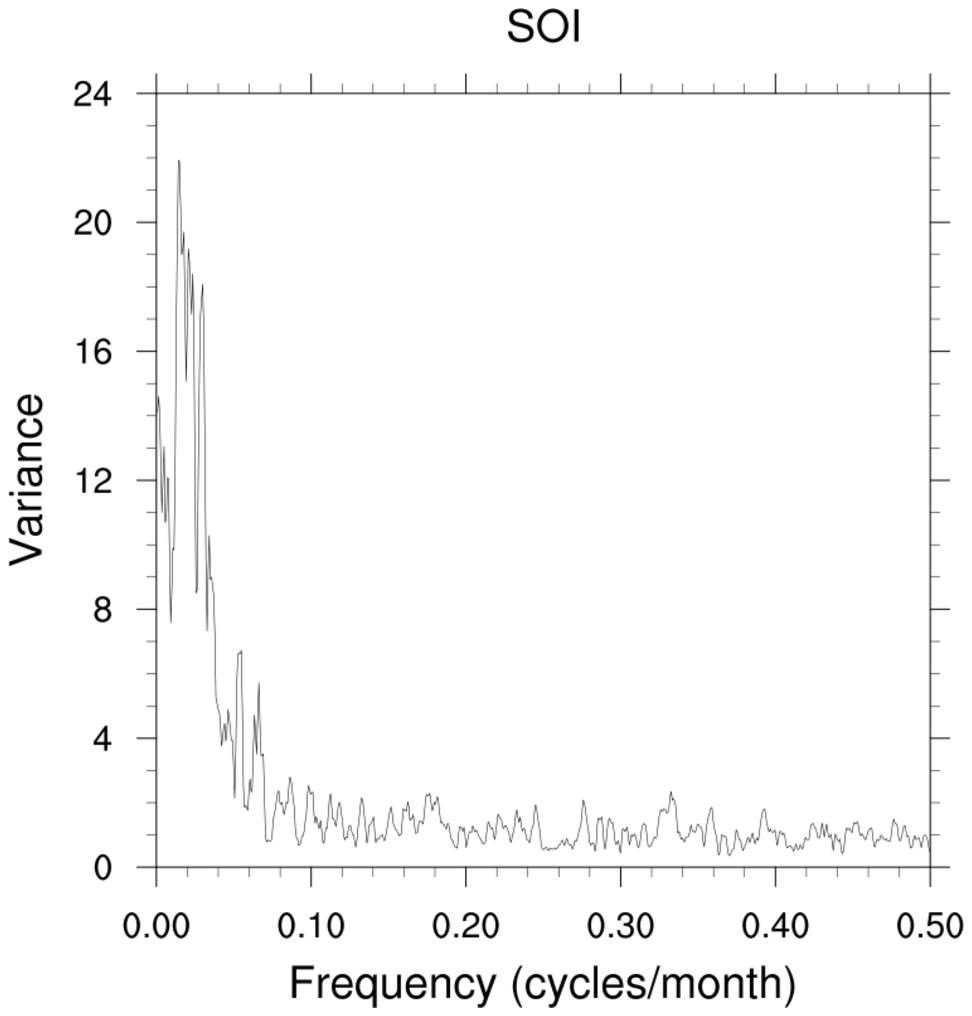
spec_2.ncl: Reads in two time series and calculates their spectra, cospectra, coherence, quadrature spectra, and phase and creates a panel plot of all values.

specxy_anal: Calculates the cospectra, coherence-squared, quadrature spectra, and phase as well as the spectra of two time series with options on smoothing, demeaning, detrending, and tapering.

The coherence-squared is a statistic that can be used to examine the relation between two signals or data sets. It allows identification of significant frequency-domain correlation between the two time series. Phase estimates in the cross spectrum are only useful where significant frequency-domain coherence-squared exists. The 6.4.0 release contains two functions that can be used to test for significance: cohsq_c2p and cohsq_p2c.

gsn_panel is the plot interface that panels plots together. More examples of panel plots.

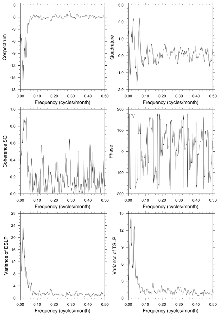
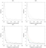spec_3.ncl: Calculates red noise confidence intervals and creates several plot variations.

specx_ci calculates a red noise confidence interval. This function returns four curves: the calculated spectrum, the "red noise" curve and the curves indicating the upper and lower confidence bounds.

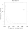
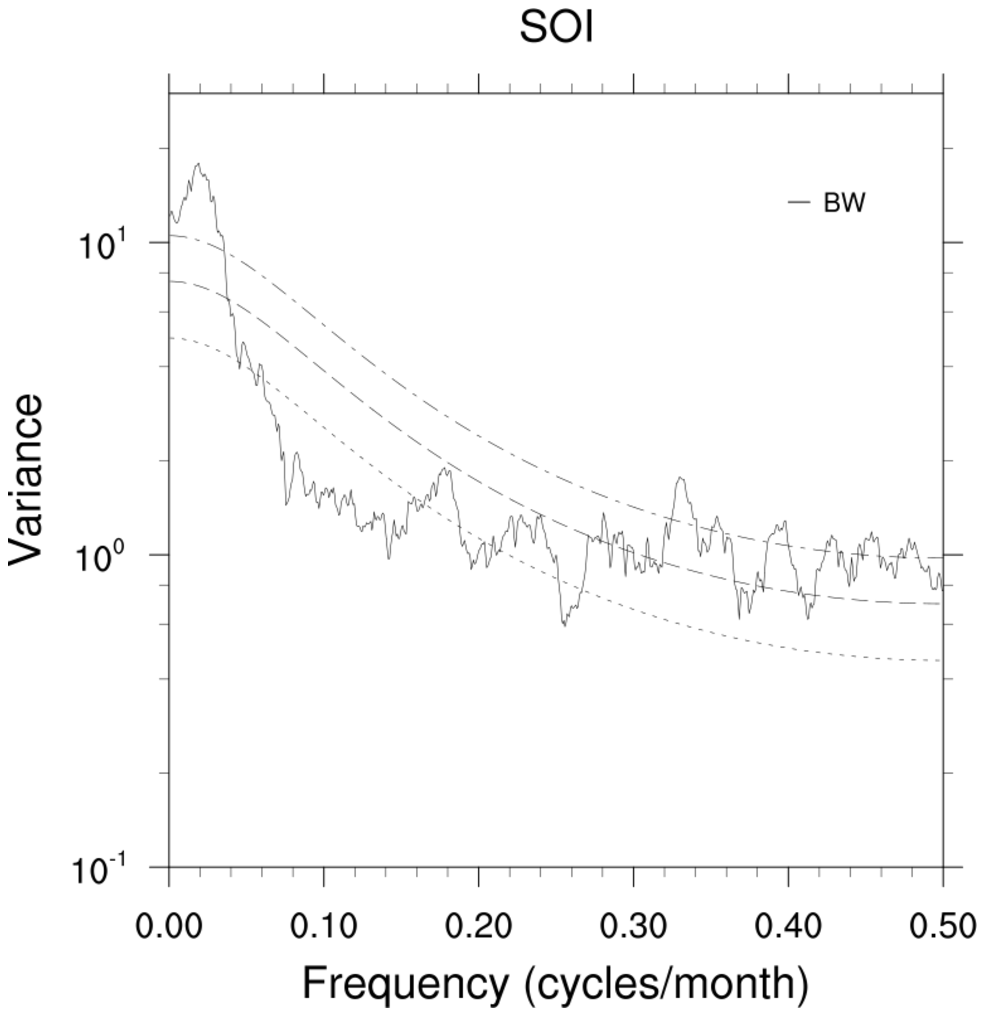
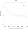spec_4.ncl: Plots spectra and "red noise" confidence intervals on a log scale and draws the bandwidth.

trYLog = True
trYMinF = 0.10
trYMaxF = 30.0, Changes the Y-axis to log and manually sets the lower adn uppe limits.

gsn_polyline and gsn_text are used to add the bandwidth line and label to the figure.

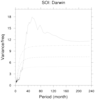
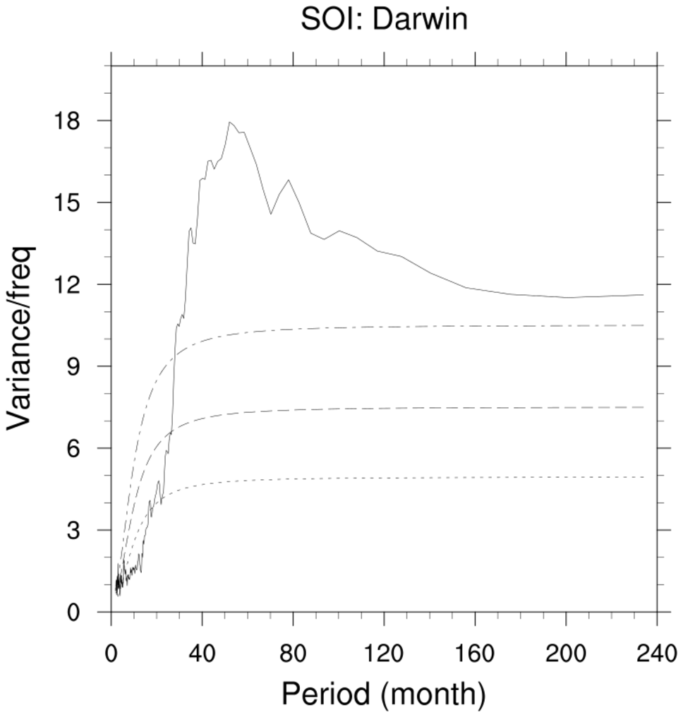
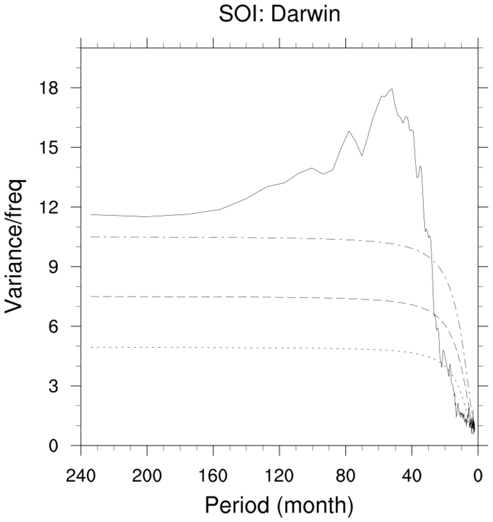
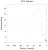spec_5.ncl: A variation of Example 4. The leftmost plot uses frequency as the abscissa. The two rightmost plots use period (1/fequency) as the abscissa. Since the period is not linear, plotting a subset of all the periods may be more useful. The ind function is used to select the desired indices. The rightmost plot illustrates how to reverse the abscissa order.

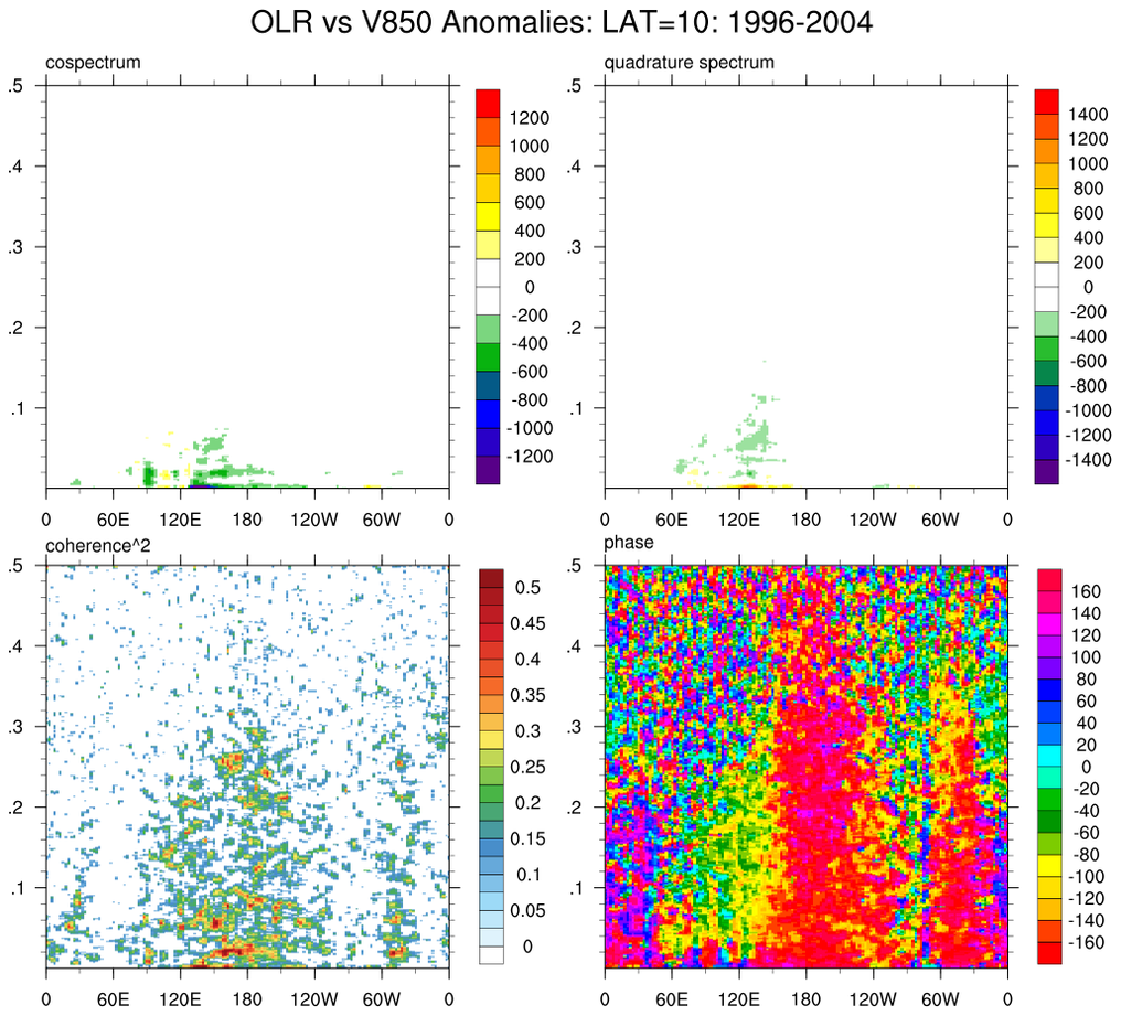
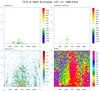CrosSpc_TimeLon_1.ncl: Calculate and plot the cross-spectral components: cospectrum, quadrature spectrum, coherence-squared and phase. Specifically, a fixed latitude [LAT] is specifed and specxy_anal is applied at each longidude to anomalies. The cross-spectral components are stored and ploted as a contour plot. The frequency unit is cycles/day.

Complex Demodulation:

As noted by Bloomfield (1976, 2000) "not all 'periodic' phenomena have simple representations in terms of cosine functions. Complex demodulation is a more flexible approach to the analysis of such data. By trading off some frequency resolution for time resolution, complex demodulation can describe features of data that would be missed by harmonic analysis. The price of this flexibility is loss of precision in describing pure frequencies, for which harmonic analysis is most exact."

Complex demodulation may be viewed as a local version of harmonic analysis. It enables the amplitude and phase of a particular frequency component of a time series to be described as functions of time. It is local in that these components are allowed to change slowly over time.

The complex demodulation process, implemented by demod_cmplx, consists of several steps:

   (1) A demodulation frequency (frqdem) is specified.
   (2) Compute the real (cosine) and imaginary (sine) components at each time step.
   (3) Low pass filter each component using a specified low pass 
       cutoff frequency (frqcut).  
   (4) Compute the amplitudes [ A(t) ] and phases [ P(t) ] 
       using the low pass filtered components (3).

The phases returned in step (4) are calculated via atan2 and range from -pi to +pi. These are called 'wrapped phases.' Unfortunately, the resulting phase plots may appear quite noisy and are difficult to interpret. For graphical and interpretation purposes, the wrapped phases are often unwrapped. NCL's unwrap_phase can be used to perform this task.

Further, as suggested by the S-Plus demod documentation:

    To better understand the results of complex demodulation 
    several lowpass filters should be tried: the smaller the pass band, 
    the less instantaneous in time but more specific in frequency is the result.

In fact, complex demodulation (like spectral analysis), could be viewed to be as much 'art' as 'science'. Different frqcut and nwt and, in some cases (Example demod_cmplx_2), different

References:

    Fourier Analysis of Time Series
    Peter Bloomfield
    Wiley, 2000

    WWW:
    http://faculty.washington.edu/kessler/generals/complex-demodulation.pdf
    http://www.pmel.noaa.gov/maillists/tmap/ferret_users/fu_2007/pdfHMANlJLqCE.pdf

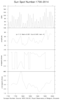
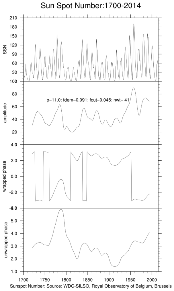
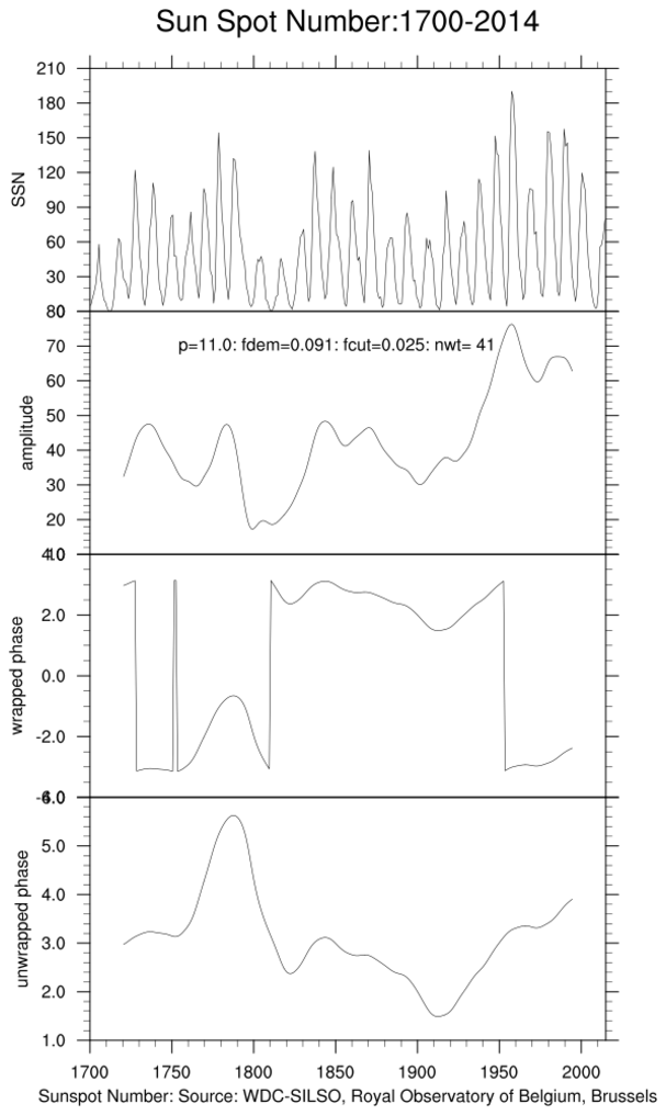
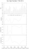demod_cmplx_1.ncl: Demodulate Wolf's annual sun spot series using NCL's demod_cmplx function. The modulation period used is 11 years [frqdem=(1.0/11)].

As noted above, several different low pass (frqcut, nwt) filters should be tried. The left figure uses frqcut=0.045 (=0.5*frqdem); the right figure uses frqcut=0.025. In both figures, the nwt=41 is kept constant. That was what Bloomfield (1976) used for his least squares filter. However, that too could be changed to get different filter effects.

The unwrapped phases created by unwrap_phase are at the bottom of the figure.

Note: frqcut and frqdem are not related. The use of frqcut=0.5*frqdem in the example (left figure) was an experiment.

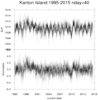
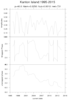
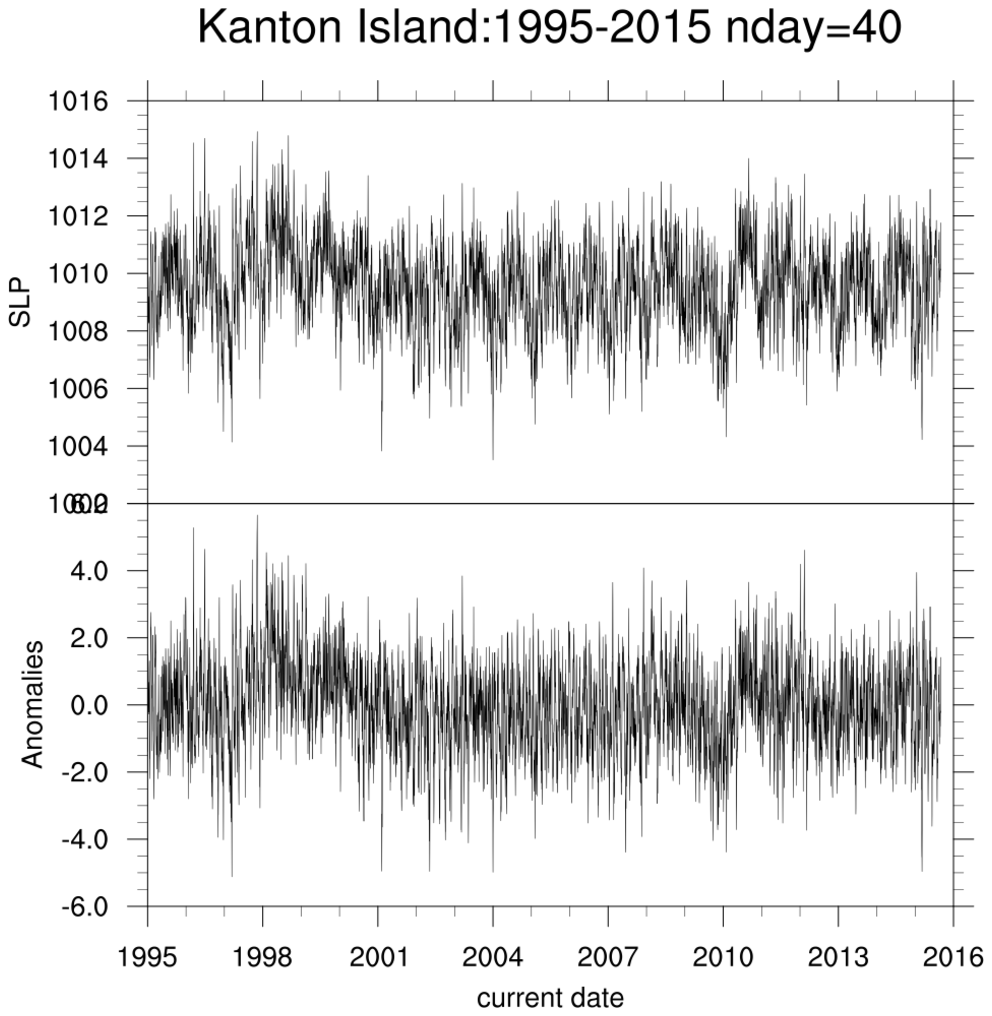
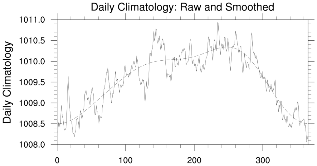
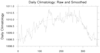
demod_cmplx_2.ncl: Read and unpack daily sea-level-pressures (slp) from grid points surrounding Kanton Island (2.8N, 188.325E). Perform a simple areal average at each time step. Calculate daily anomalies from a daily climatology. Perform a complex demodulation on the anomaly time series about a period of 40 days (frqdem=(1/40). Commonly, the Madden-Julian Oscillation (MJO) is described as having a 30-60 day period.

Since the MJO spans 30-60 days several different demodulation (frqdem) frequencies should be examined. Again, different frqcut and nwt should be examined.

The unwrapped phases created by unwrap_phase are at the bottom of the middle figure.