NCL Home > Documentation > Functions > General applied math

specx_ci

Calculates the theoretical Markov spectrum and the lower and upper confidence curves.

Prototype

load "$NCARG_ROOT/lib/ncarg/nclscripts/csm/gsn_code.ncl"      ; These four libraries are automatically
load "$NCARG_ROOT/lib/ncarg/nclscripts/csm/gsn_csm.ncl"       ; loaded from NCL V6.4.0 onward.
load "$NCARG_ROOT/lib/ncarg/nclscripts/csm/contributed.ncl"   ; No need for user to explicitly load.
load "$NCARG_ROOT/lib/ncarg/nclscripts/csm/shea_util.ncl"

	function specx_ci (
		sdof [1] : numeric,  
		lowval   : numeric,  
		highval  : numeric   
	)

	return_val [4][*] :  typeof(sdof)

Arguments

sdof

A degrees-of-freedom array returned from the NCL functions specx_anal or specxy_anal.

lowval

The lower confidence limit (0.0 < lowval < 1.). A typical value is 0.05.

highval

The upper confidence limit (0.0 < hival < 1.). A typical value is 0.95.

Return value

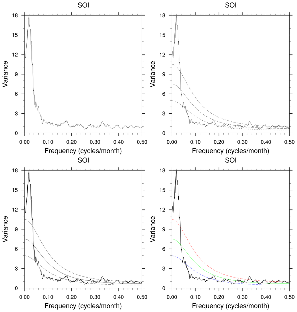
A two-dimensional array dimensioned 4 x N where N is the size of sdof@spcx. It will contain four curves:

• splt(0,:) - input spectrum
• splt(1,:) - Markov "Red Noise" spectrum
• splt(2,:) - lower confidence bound for Markov
• splt(3,:) - upper confidence bound for Markov

Description

This function calculates the theoretical Markov spectrum and the lower and upper confidence curves using the lag-1 autocorrelation returned as an attribute by the NCL functions specx_anal or specxy_anal.

See Also

specx_anal, specxy_anal

Examples

Example 1

Sample usage

load "$NCARG_ROOT/lib/ncarg/nclscripts/csm/gsn_code.ncl" 
load "$NCARG_ROOT/lib/ncarg/nclscripts/csm/gsn_csm.ncl" 
load "$NCARG_ROOT/lib/ncarg/nclscripts/csm/contributed.ncl"
load "$NCARG_ROOT/lib/ncarg/nclscripts/csm/shea_util.ncl"

begin
  f      = addfile ("/cgd/cas/shea/MURPHYS/ATMOS/b003_T_200-299.nc", "r")
  x      = f->T(:,17,:,:)
  x = rmMonAnnCycTLL(x)   ;removes the annual cycle from monthly data, in contributed.ncl
  ts = x(:,{50.},{290.})

  sdof = specx_anal(ts,0,0,0.1)
  splt = specx_ci(sdof,0.05,0.95)
  
  wks = gsn_open_wks("ps","test")
  res                     = True
  res@tiYAxisString = "Power"              ; yaxis
  res@xyLineThicknesses   = (/2.,1.5,1.,1./)  ; Define line thicknesses 
  res@xyDashPatterns      = (/0,0,0,0/)
  res@xyLineColors        = (/"foreground","red","blue","green"/)                

  plot = gsn_csm_xy(wks,sdof@frq,splt,res)
end

For some application examples, see:

• "spec_3.ncl" (view example)
• "spec_4.ncl" (view example)

Example 2

Compute the mean spectrum and confidence intervals from an ensemble of time segments. Let x(nseg,ntim) where 'nseg' is the number of number of temporal segments and 'ntim' is the length of each segment.

   d   = 0
   sm  = 1         ; periodogram
   pct = 0.10

  ;************************************************
  ; calculate mean spectrum spectrum and lag1 auto cor
  ;************************************************
  
  ; loop over each segment of length ntim
  
   spcavg = new ( ntim/2, typeof(x))
   spcavg = 0.0
  
   r1zsum = 0.0
  
   do n=0,nseg-1
      dof    = specx_anal(x(n,:),d,sm,pct)      ; current segment spc
      spcavg = spcavg + dof@spcx                ; sum spc of each segment
      r1     = dof@xlag1                        ; extract segment lag-1
      r1zsum = r1zsum  + 0.5*(log((1+r1)/(1-r1)) ; sum the Fischer Z
   end do
  
   r1z  = r1zsum/nseg                           ; average r1z
   r1   = (exp(2*r1z)-1)/(exp(2*r1z)+1)            ; transform back
                                                ; this is the mean r1
   spcavg  = spcavg/nseg                        ; average spectrum
  
  ;************************************************
  ; Assign mean spectrum to data object
  ;************************************************
  
   df      = 2.0*nseg                           ; deg of freedom
                                                ; all segments
   df@spcx = spcavg                             ; assign the mean spc
   df@frq  = dof@frq
   spcavg@xlag1 = r1                            ; assign mean lag-1
  
  ;************************************************
  ; plotting
  ;************************************************
    wks  = gsn_open_wks("ps","spec")              ; Opens a ps file

    res = True
    res@tiMainString = "Mean Spectra: "+nseg+" segments, dof="+df                   ; title
    res@tiXAxisString = "Frequency (cycles/month)"  ; xaxis
    res@tiYAxisString = "Variance"                  ; yaxis

    splt = specx_ci(df, 0.05, 0.95)                 ; confidence interval

    plot = gsn_csm_xy(wks, df@frq, splt ,res)      ; create plot
					

Contact the Webmaster