NCL Home>
Application examples>
Plot techniques ||
Data files for some examples
Example pages containing:
tips |
resources |
functions/procedures
NCL Graphics: Tables and gridded cells
You can draw basic tables in NCL using the
gsn_table procedure.
To draw plots of gridded cells, you can use
gsn_csm_blank_plot
to create a blank plot, and then call
gsn_add_polygon and
gsn_add_polyline
to add filled polygons and lines.
To annotate a plot with labelbars or text, use
use gsn_create_labelbar
gsn_add_annotation,
and/or gsn_add_text.
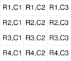
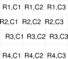 table_1.ncl
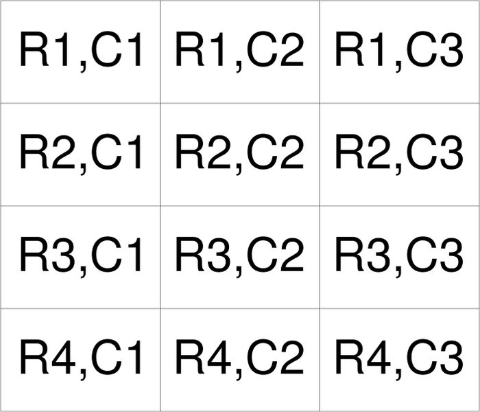
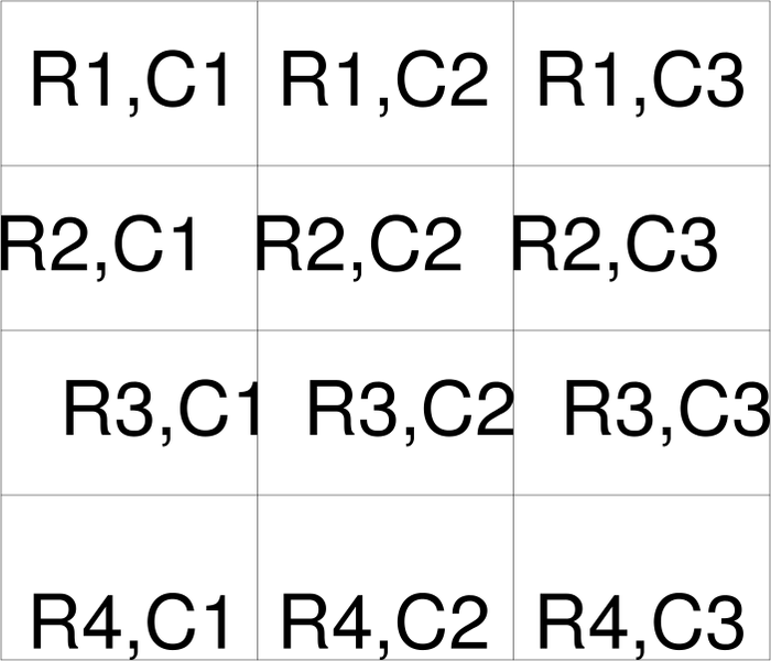
:
Example of a simple table
using
gsn_table. This table has 4
rows and 3 columns. No resources are set in the first frame, and then
the second frame sets
txJust to
control the justification of the text (the default is "CenterCenter").
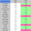 table_2.ncl
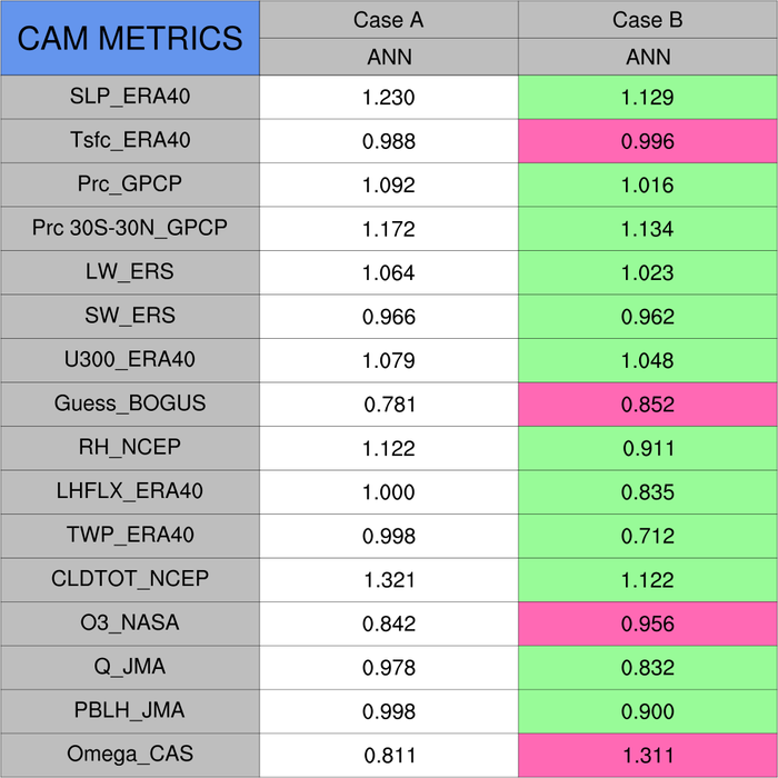
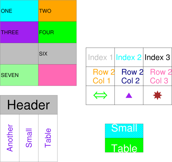
:
This table is actually made up of three separate tables. It is a
duplicate of the one found on the
taylor
applications page.
The gsFillColor resource is
used to fill the grid cells. In order to get a different fill color
for various cells, this resource is set to an array of the same size
as the text strings, and given a fill color for every cell.
A Python version of this projection is available here.
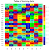 table_4.ncl
:
This example shows how to associate tickmarks with a table.
The
gsn_csm_blank_plot function
is used to create a blank plot, and then we draw the
table in the same location. We also attach a separate
labelbar using
gsn_create_labelbar
and
gsn_add_annotation. We had to set
the vpXXXX resources for the blank plot to make sure we left room to
add the labelbar on the outside.
This example reads dummy data from
the table4.txt file.
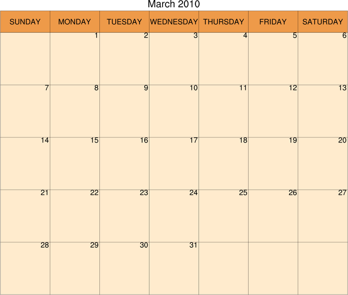
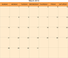 table_5.ncl
:
This example shows how to use
gsn_table
to create a monthly calendar. Each calendar contains
three tables: the main title, the day of the week heading, and the
days of the month. The position of each table is determined by using
position information from the previous table.
Command line options can be used to indicate how the calendar(s) are
to be generated:
- Calendar for current month and year:
ncl table_5.ncl
- Calendar for a particular month:
ncl month=10 table_5.ncl
- Calendar for a particular month and year:
ncl month=9 year=2010 table_5.ncl
- All calendars for the current year:
ncl ALL_MONTHS=True table_5.ncl
- All calendars for a given year:
ncl ALL_MONTHS=True year=2011 table_5.ncl
 indices_oni_1.ncl
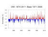
:
NOAA's operational definitions of El Niño and La Niña conditions are based
upon the
Oceanic Niño Index [
ONI]. The ONI is defined as
the
3-month running means of SST anomalies in the Niño 3.4
region [5N-5S, 120-170W]. The anomalies
are derived from the 1971-2000 SST climatology.
The Niño 3.4 anomalies may be thought of as representing the average equatorial
SSTs across the Pacific from about the dateline to the South American coast.
To be classified as a full-fledged El Niño and La Niña episode the ONI must exceed
+0.5 [El Niño] or -0.5 [La Niña] for at least five consecutive months.
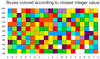
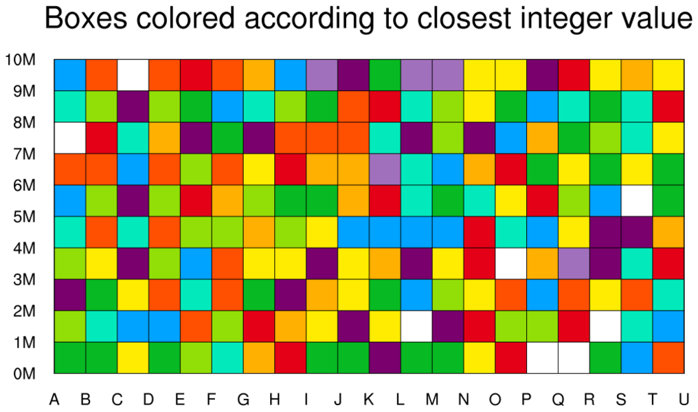
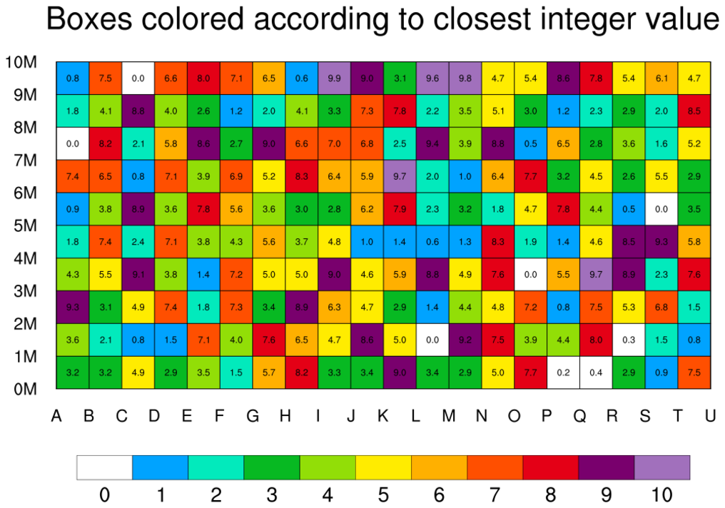
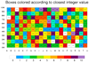 table_7.ncl
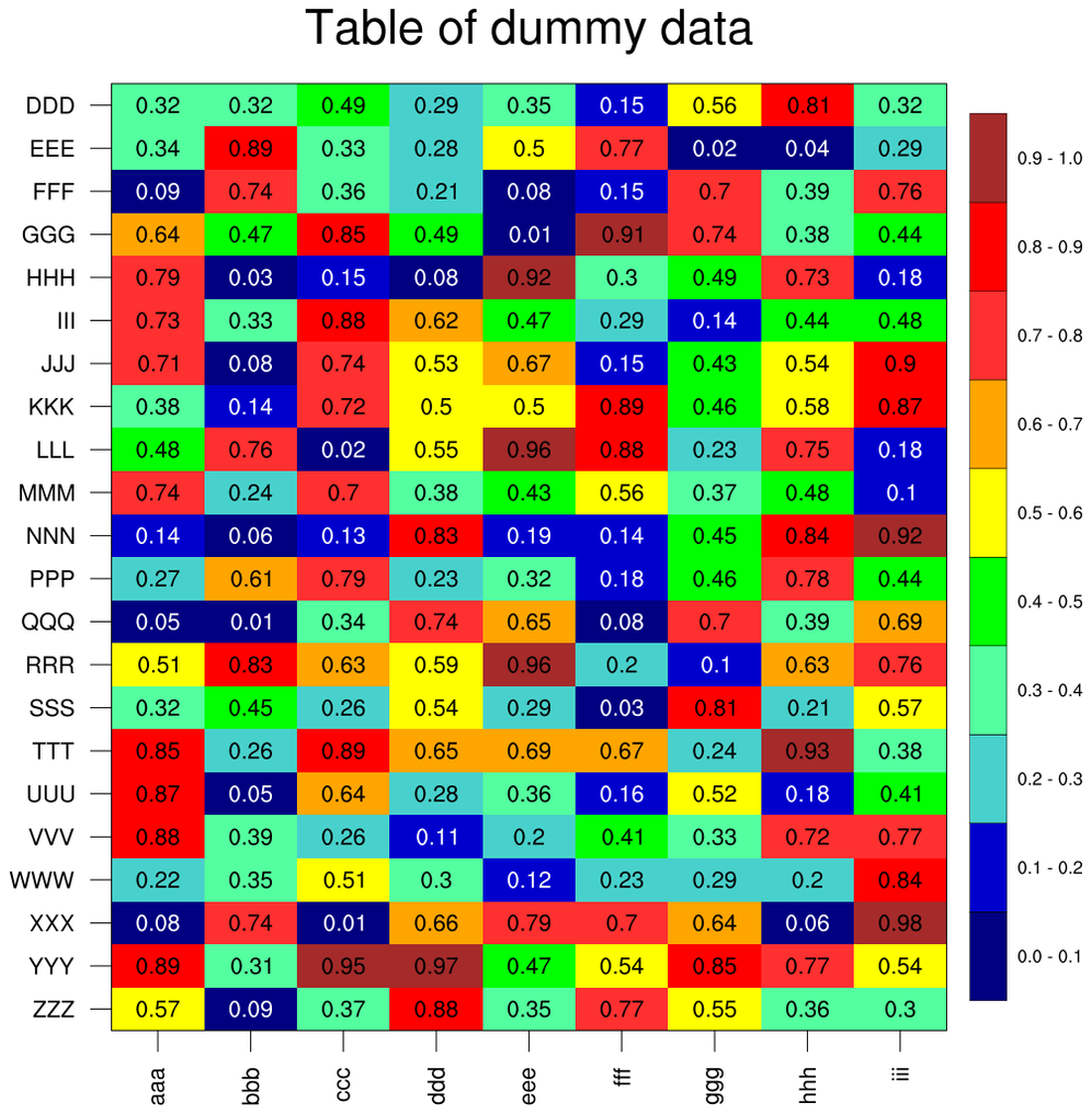
: This script
shows how to draw filled gridded cells using
gsn_csm_blank_plot
and
gsn_add_polygon.
The closest_val
function is used to find the closest integer value to
each data value, and that cell is then filled in the
appropriate color.
The second frame shows how to annotate the plot using
gsn_create_labelbar
for a labelbar and gsn_add_text
for text strings.
This script is based on one written by Yang Zhao
of the Chinese Academy of Meteorological Sciences.
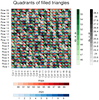
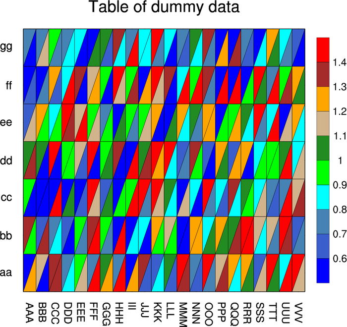
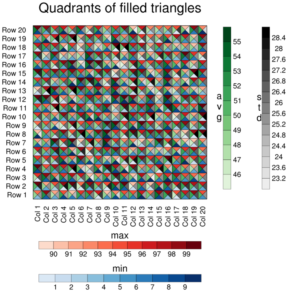
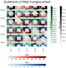 table_8.ncl
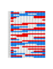
:
This example is similar to table_6.ncl, except it draws four triangles
per each quadrant. The bottom triangles represent the minimum of the
values, the top triangles represent the maximum of the values, the
left triangles represent the average, and the right triangles the
standard deviation. Each set of triangles has their own color map,
illustrated by the four labelbars.
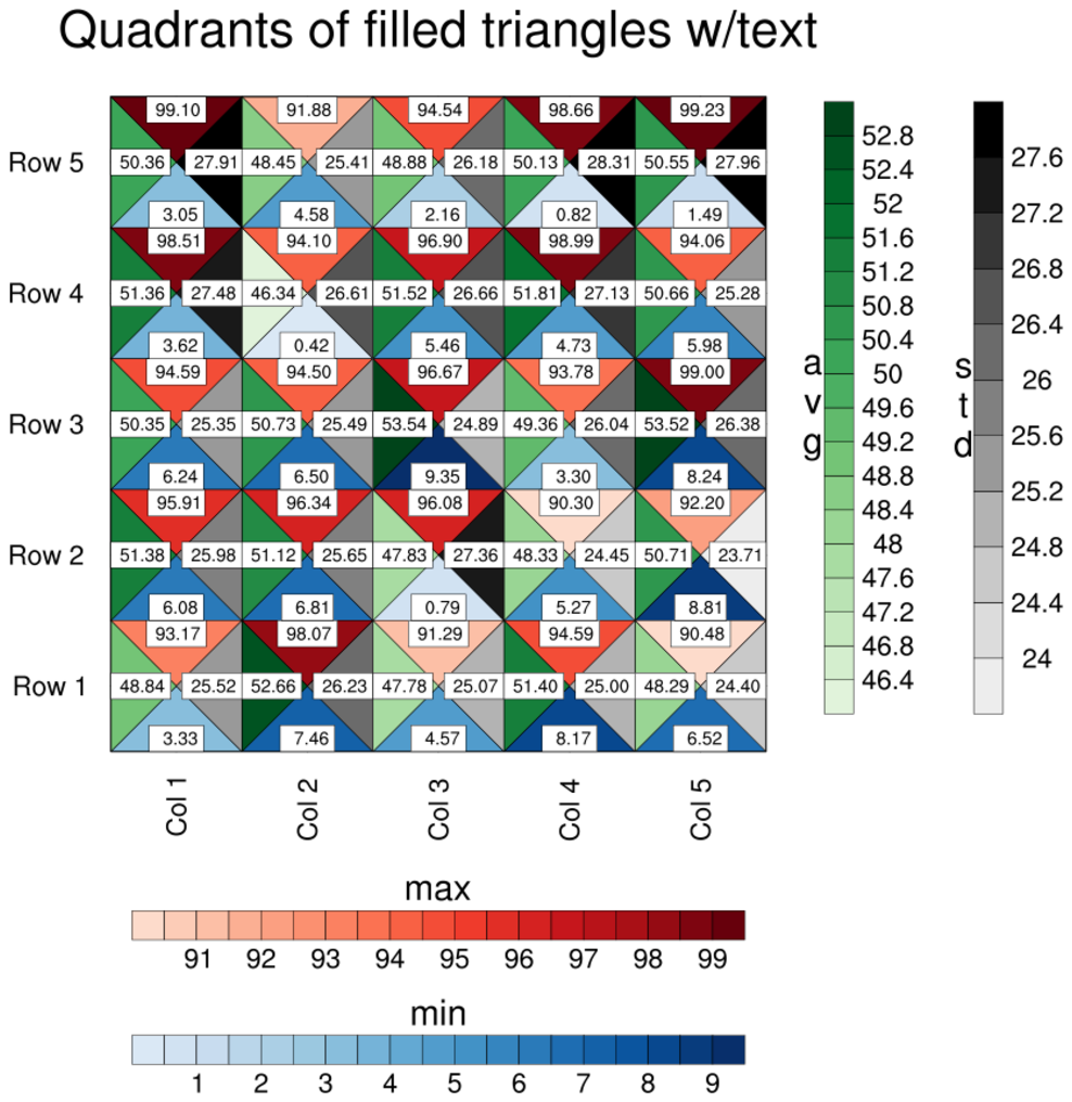
The second image is from running the script with nvars=5, nmodels=5, and ADD_TEXT=True.
This is just for debugging purposes, so you can see what each triangle value is equal
to.
Dummy data is used, which is generated by the script.

