See the time axis labels page for examples of creating nice time labels on the X or Y axis.
NCL Home>
Application examples>
Data Analysis ||
Data files for some examples
 time_3.ncl: Demonstrates what
happens if you try to plot a time series plot with YYYYMM values on the
X axis. NCL has no way of knowing this is a time axis, so it treats
the YYYYMM values as being on a linear axis, and includes values YYYY13,
YYYY14, through YYYY99, causing irregular gaps in the data.
time_3.ncl: Demonstrates what
happens if you try to plot a time series plot with YYYYMM values on the
X axis. NCL has no way of knowing this is a time axis, so it treats
the YYYYMM values as being on a linear axis, and includes values YYYY13,
YYYY14, through YYYY99, causing irregular gaps in the data.
 time_4.ncl: Demonstrates how to use the
contributed.ncl function
yyyymm_to_yyyyfrac to set up
a monthly time array useful for plotting purposes. The top panel
shows a random-generated timeseries plotted along an X-axis set up
using yyyymm_to_yyyyfrac. The
middle plot shows the result of
using tmXBFormat to remove unnecessary
trailing zeros from the X axis labels.
The bottom panel shows how to include carriage
returns in tick mark labels so that the year label appears under the month label.
time_4.ncl: Demonstrates how to use the
contributed.ncl function
yyyymm_to_yyyyfrac to set up
a monthly time array useful for plotting purposes. The top panel
shows a random-generated timeseries plotted along an X-axis set up
using yyyymm_to_yyyyfrac. The
middle plot shows the result of
using tmXBFormat to remove unnecessary
trailing zeros from the X axis labels.
The bottom panel shows how to include carriage
returns in tick mark labels so that the year label appears under the month label.
Example pages containing: tips | resources | functions/procedures
Time coordinates
This page shows some examples of dealing with "time" coordinates.
All "date" functions are documented here.
CAUTION:
The yyyy-mm within a CESM file name and the time variable
contained within the file may not necessarily agree with one another. This can
be confusing and lead to erroneous temporal assignment(s). Consider a file named
"CESM.sample.h.0280-01.nc". The file 'yyyy-mm' is 280-01 (January, 280).
 f = addfile("CESM.sample.h.0280-01.nc","r")
 time = f->time
 print(time)

     Variable: time
     Type: double
              [snip]
     Dimensions and sizes:	[time | 1]
     Coordinates:
              time: [102231..102231]
     Number Of Attributes: 4
       long_name :	time
     units :	days since 0000-01-01 00:00:00
     bounds :	time_bound
     calendar :	noleap

     (0)     102231

 date = cd_calendar(time, 0)
 print(date)

     Variable: date
     Dimensions and sizes:   [1] x [6]     <== yyyy,mm,dd,hh,mn,sec
     Coordinates:
     Number Of Attributes: 1
     calendar :    noleap
    (0,0)   280
    (0,1)    2
              [snip]
The variable 'time' indicates 280-02 or February, 280 which is not consistent with the file name of 280-01 or January, 280. How to deal with this? One approach is to use the 'time_bound' variable.
 time_bound = f->time_bound
 print(time_bound)

     Variable: time_bound
     Type: double
     Total Size: 16 bytes
                 2 values
     Number of Dimensions: 2
     Dimensions and sizes:   [time | 1] x [d2 | 2]
     Coordinates:
                 time: [102231..102231]
     Number Of Attributes: 2
       long_name :   boundaries for time-averaging interval
       units :       days since 0000-01-01 00:00:00

  (0,0)   102200     <==== beginning of the averaging time
  (0,1)   102231     <==== this is the same as 'time'

 time = (/ time_bound(:,0) /)          ; override values with lower bound
 print(time)                           ; <=== 102200
 date = cd_calendar(time, 0)
 print(date)

     Variable: date
     Type: float
     Total Size: 24 bytes
                 6 values
     Number of Dimensions: 2
     Dimensions and sizes:   [1] x [6]
     Coordinates:
     Number Of Attributes: 1
       calendar :    noleap
  (0,0)   280
  (0,1)    1

------------------------------------------------------------------------------>
------------------------------------------------------------------------------>
Another (better ?) approach is to average the time_bnd variable to get the
'center-of-mass' of the observations.

 time       = f->time
 time_bound = f->time_bound
 time       = (/ (time_bound(:,0)+time_bound(:,1))*0.5 /)  ; replace values with average

For NCL applications, one could reassign the 'time' coordinate variable
associated with a variable:

 temp       = f->TEMP
 temp&time  = (/ time  /)     ; reasign with 'center-of-mass' time values
time_1.ncl: (a) Create an integer time
coordinate variable of the type 199801,199802 etc
for multiple years. (b) Convert to type string via tostring
and sprinti. (c) Convert integer yyyymm to year and fraction
of year for graphics via yyyymm_to_yyyyfrac.
(d) Create a time variable with the units "hours since ...".
                yyyymm    _s1     _s2     time    yrfrac

          (0)	199801  199801  199801   859032   1998
          (1)	199802  199802  199802   859776   1998.08
          (2)	199803  199803  199803   860448   1998.17
          (3)	199804  199804  199804   861192   1998.25
          (4)	199805  199805  199805   861912   1998.33
          (5)	199806  199806  199806   862656   1998.42
          (6)	199807  199807  199807   863376   1998.5
          (7)	199808  199808  199808   864120   1998.58
          (8)	199809  199809  199809   864864   1998.67
          (9)	199810  199810  199810   865584   1998.75
          (10)	199811  199811  199811   866328   1998.83
          (11)	199812  199812  199812   867048   1998.92
          (12)	199901  199901  199901   867792   1999

          [SNIP]

          (35)	200012  200012  200012   884592   2000.92
          (36)	200101  200101  200101   885336   2001
          (37)	200102  200102  200102   886080   2001.08
          (38)	200103  200103  200103   886752   2001.17
          (39)	200104  200104  200104   887496   2001.25
          (40)	200105  200105  200105   888216   2001.33
          (41)	200106  200106  200106   888960   2001.42
          (42)	200107  200107  200107   889680   2001.5
          (43)	200108  200108  200108   890424   2001.58
          (44)	200109  200109  200109   891168   2001.67
          (45)	200110  200110  200110   891888   2001.75
          (46)	200111  200111  200111   892632   2001.83
          (47)	200112  200112  200112   893352   2001.92
time_2.ncl: Demonstrates using
cd_calendar to convert a mixed Julian/Gregorian
date to a UT-referenced date, and then demonstrates using
cd_inv_calendar to go from
a UT-referenced date to a mixed Julian/Gregorian date with a different
reference time and units. The sprintf is used to
ensure consistent formatting of the yrfrac variable.
          Variable: time                            ; original 'time'
          Type: double
          Total Size: 6560 bytes
                      820 values
          Number of Dimensions: 1
          Dimensions and sizes:   [time | 820]
          Coordinates:
                      time: [1297320..1895592]             ; range of values
          Number Of Attributes: 7
            long_name :   Time
            delta_t :     0000-01-00 00:00:00
            prev_avg_period :     0000-00-01 00:00:00
            standard_name :       time
            axis :        T
            units :       hours since 1800-01-01 00:00:0.0 ; reference time
            actual_range :        ( 1297320, 1895592 )

          -----

          Variable: time2
          Type: double
          Total Size: 6560 bytes
                      820 values
          Number of Dimensions: 1
          Dimensions and sizes:   [time2 | 820]
          Coordinates:
                      time2: [53690..78618]                 ; new reference range
          Number Of Attributes: 2
            calendar :    standard
            units :       days since 1801-1-1 00:00:0.0     ; new reference units

OUTPUT:

                   time    yyyymm  yyyymmdd  yyyymmddhh  yyyy.frac  time2
          (0)     1297320  194801  19480101  1948010100  1948.0000  53690
          (1)     1298064  194802  19480201  1948020100  1948.0847  53721
          (2)     1298760  194803  19480301  1948030100  1948.1639  53750
          (3)     1299504  194804  19480401  1948040100  1948.2486  53781
          (4)     1300224  194805  19480501  1948050100  1948.3306  53811
          (5)     1300968  194806  19480601  1948060100  1948.4153  53842
          (6)     1301688  194807  19480701  1948070100  1948.4973  53872

          [SNIP]

          (812)   1890480  201509  20150901  2015090100  2015.6658  78405
          (813)   1891200  201510  20151001  2015100100  2015.7479  78435
          (814)   1891944  201511  20151101  2015110100  2015.8329  78466
          (815)   1892664  201512  20151201  2015120100  2015.9151  78496
          (816)   1893408  201601  20160101  2016010100  2016.0000  78527
          (817)   1894152  201602  20160201  2016020100  2016.0847  78558
          (818)   1894848  201603  20160301  2016030100  2016.1639  78587
          (819)   1895592  201604  20160401  2016040100  2016.2486  78618
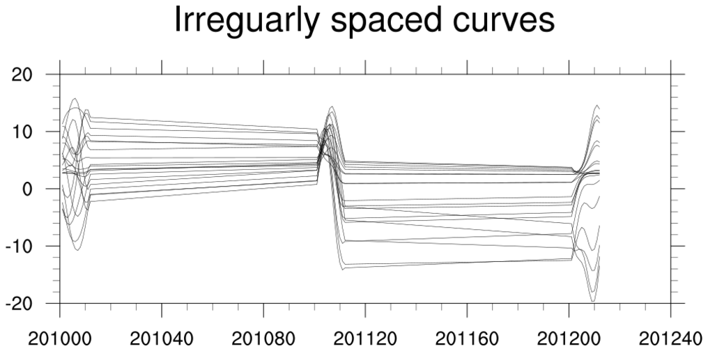
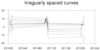
 time_3.ncl: Demonstrates what
happens if you try to plot a time series plot with YYYYMM values on the
X axis. NCL has no way of knowing this is a time axis, so it treats
the YYYYMM values as being on a linear axis, and includes values YYYY13,
YYYY14, through YYYY99, causing irregular gaps in the data.
time_3.ncl: Demonstrates what
happens if you try to plot a time series plot with YYYYMM values on the
X axis. NCL has no way of knowing this is a time axis, so it treats
the YYYYMM values as being on a linear axis, and includes values YYYY13,
YYYY14, through YYYY99, causing irregular gaps in the data.
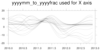
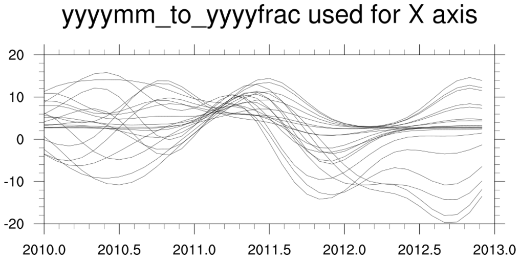
To fix this, you can use the function yyyymm_to_yyyyfrac to convert YYYYMM to yearly fractional values. The second plot illustrates the use of this function.
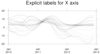
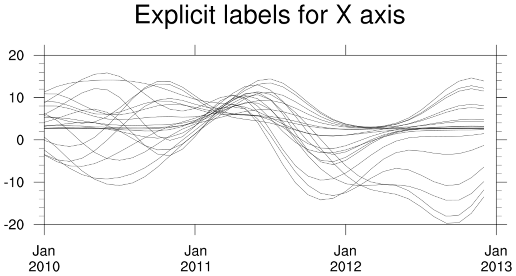
The third plot simply shows how to label the X axis with more meaningful time labels.
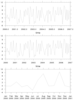
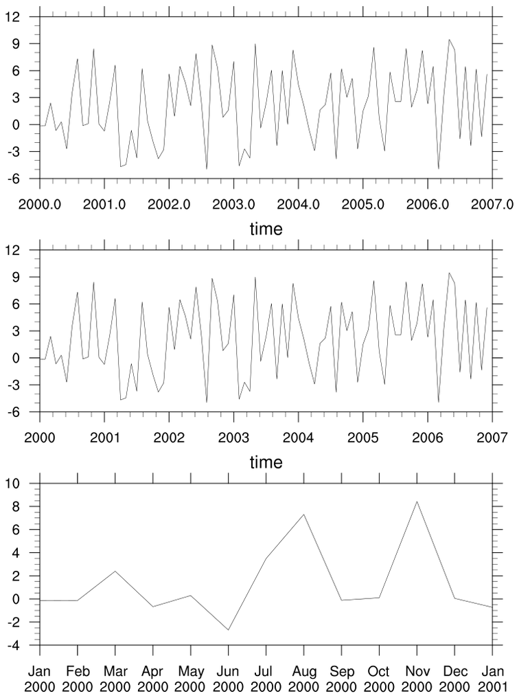 time_4.ncl: Demonstrates how to use the
contributed.ncl function
yyyymm_to_yyyyfrac to set up
a monthly time array useful for plotting purposes. The top panel
shows a random-generated timeseries plotted along an X-axis set up
using yyyymm_to_yyyyfrac. The
middle plot shows the result of
using tmXBFormat to remove unnecessary
trailing zeros from the X axis labels.
The bottom panel shows how to include carriage
returns in tick mark labels so that the year label appears under the month label.
time_4.ncl: Demonstrates how to use the
contributed.ncl function
yyyymm_to_yyyyfrac to set up
a monthly time array useful for plotting purposes. The top panel
shows a random-generated timeseries plotted along an X-axis set up
using yyyymm_to_yyyyfrac. The
middle plot shows the result of
using tmXBFormat to remove unnecessary
trailing zeros from the X axis labels.
The bottom panel shows how to include carriage
returns in tick mark labels so that the year label appears under the month label.
Carriage returns are created in text strings by utilizing a text function code surrounding a C. (ex. ~C~)