NCL Graphics: Using gsn_csm scripts to plot WRF-ARW data

wrf_gsn_1.ncl / wrf_nogsn_1.ncl: The first frame is an example of plotting WRF-ARW data using gsn_csm_contour_map (wrf_gsn_1.ncl).

The second frame uses wrf_contour and wrf_map_overlays (wrf_nogsn_1.ncl).

The "HGT" variable is plotted here. This is a good variable to use for testing purposes, because it's easy see if the plot looks correct.

wrf_gsn_2.ncl: This example is similar to the previous one, except it shows how to set some more plot resources to get a slightly nicer plot.

Just for informational purposes, this script calls wrf_map_resources and prints out the resultant resource list, so you can see what map resources would normally be set by wrf_map_overlays. Here's an example of some of those resources:

  pmTickMarkDisplayMode   : "Always"
  mpOutlineBoundarySets   : "GeophysicalAndUSStates"
  mpUSStateLineThicknessF : 0.5
  mpUSStateLineColor      : "Gray"
  mpLimbLineThicknessF    : 0.5
  mpGridSpacingF          : 5
  mpGridLineThicknessF    : 0.5
  tmYLLabelFontHeightF    : 0.01

wrf_gsn_3.ncl: This example is similar to the previous one, except the map is further zoomed in on using mpMinLatF / mpMaxLatF and mpMinLonF / mpMaxLonF, and the WRF grid is drawn first as purple markers, and then as brown lines, using gsn_coordinates. This is mainly for debug purposes.

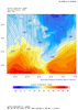
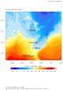
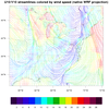
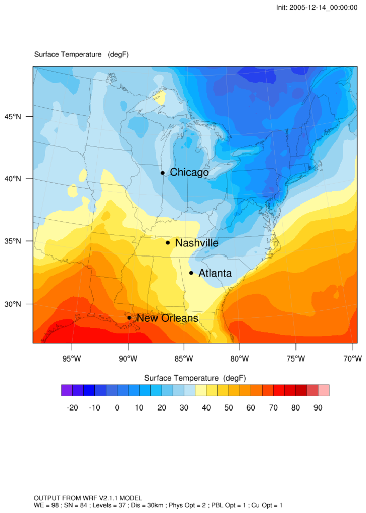
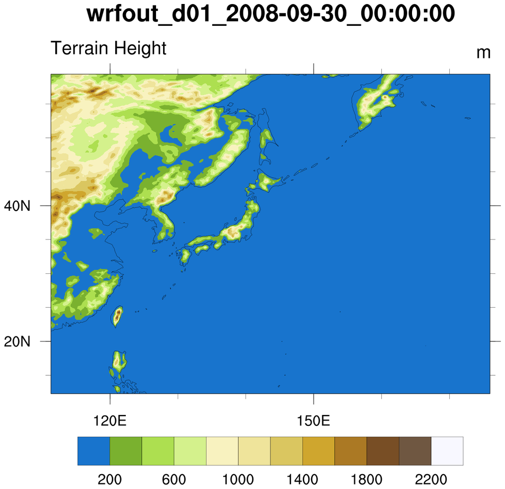
wrf_gsn_4.ncl / wrf_nogsn_4.ncl: This example shows how to plot WRF-ARW data using gsn_csm_contour_map, but using the native map projection provided on the WRF output file. The wrf_map_resources function is used to set the correct map projection resources. This can be useful if you want to use the native WRF map projection but you need more control over plot elements, like the titles or labelbar.

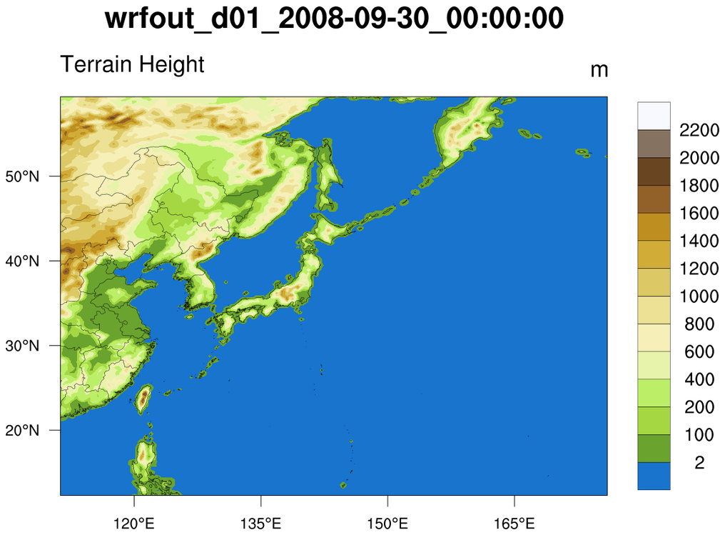
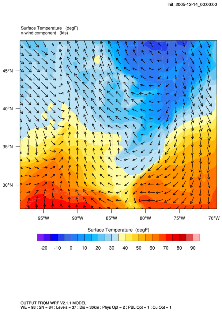
The second image is of the same variable, but plotted with wrf_contour and wrf_map_overlays. The contour levels are slightly different because wrf_contour internally increases the number of contour levels from the default NCL uses.

wrf_gsn_5.ncl / wrf_nogsn_5.ncl: This example shows how to overlay line contours, vectors, and filled contours on a map. The data and map projection are all read off a WRF output file.

The first frame shows how to do this using gsn_csm_xxx scripts, and the second frame shows how to do this using wrf_xxxx scripts.

Note that using the gsn_csm_xxxx method requires that you set many more resources to customize the plot. This is because the wrf_xxxx scripts set many of these resources for you. The reason for using gsn_csm_xxxx scripts is to give you more flexibility over setting plot options, and to use a different map projection if desired.

wrf_nogsn_poly_5.ncl: This example is similar to wrf_nogsn_5.ncl above, except it shows how to add text and markers to an existing plot that was drawn with wrf_map_overlays.

The key is to set "pltres@PanelPlot = True", telling this function that you plan to do something with the plot later. This causes wrf_map_overlays to not draw the plot and to not remove all the overlain features, allowing you to put more annotations on the plot before drawing it yourself.

gsn_add_polymarker and gsn_add_text are used to add the dots and text strings to the WRF plot.

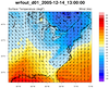
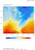wrf_gsn_6.ncl / wrf_nogsn_6.ncl: This example is similar to the previous "wrf_gsn_5.ncl" one, except it doesn't draw sea level pressure contours.

The point of this example is to show another way of drawing WRF plots. This one uses gsnLeftString and gsnRightString to title the plot, and it changes more features of the WRF map to make the map outlines more thick and prominent.

The second frame is plotting the same data, except using wrf_contour, wrf_vector, and wrf_map_overlays. Notice that with this plot, you get some very nice titling without much effort.

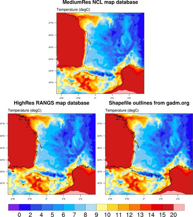
The "HighRes" map database is used to get better coastal outlines. If you want to use the "HighRes" map database, you will have to download the RANGS database.

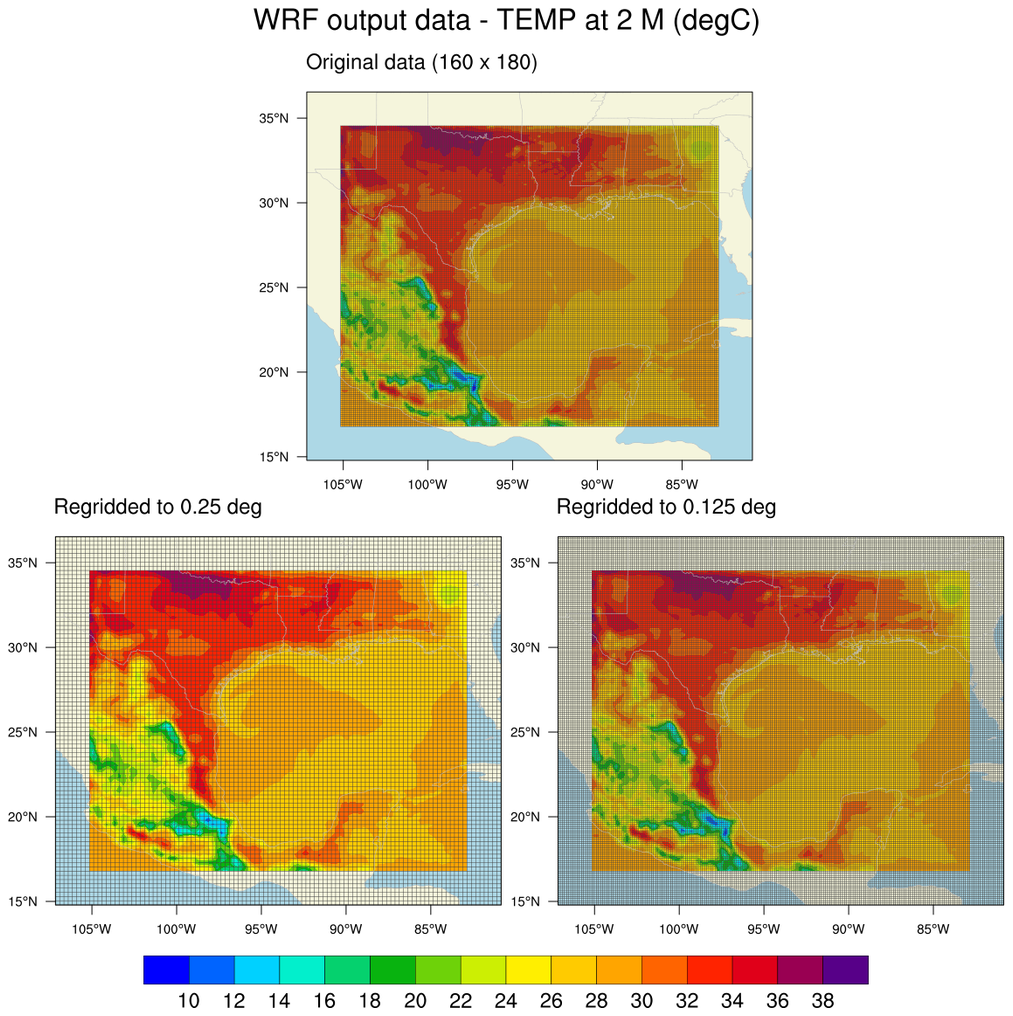
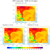
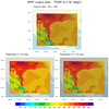
wrf_gsn_7.ncl This example regrids WRF output data to both a 0.25 and 0.125 degree grid, and compares them in a panel plot.

For the second image, the gsn_coordinates procedure was used to draw the lat/lon grid on all three plots.

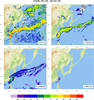
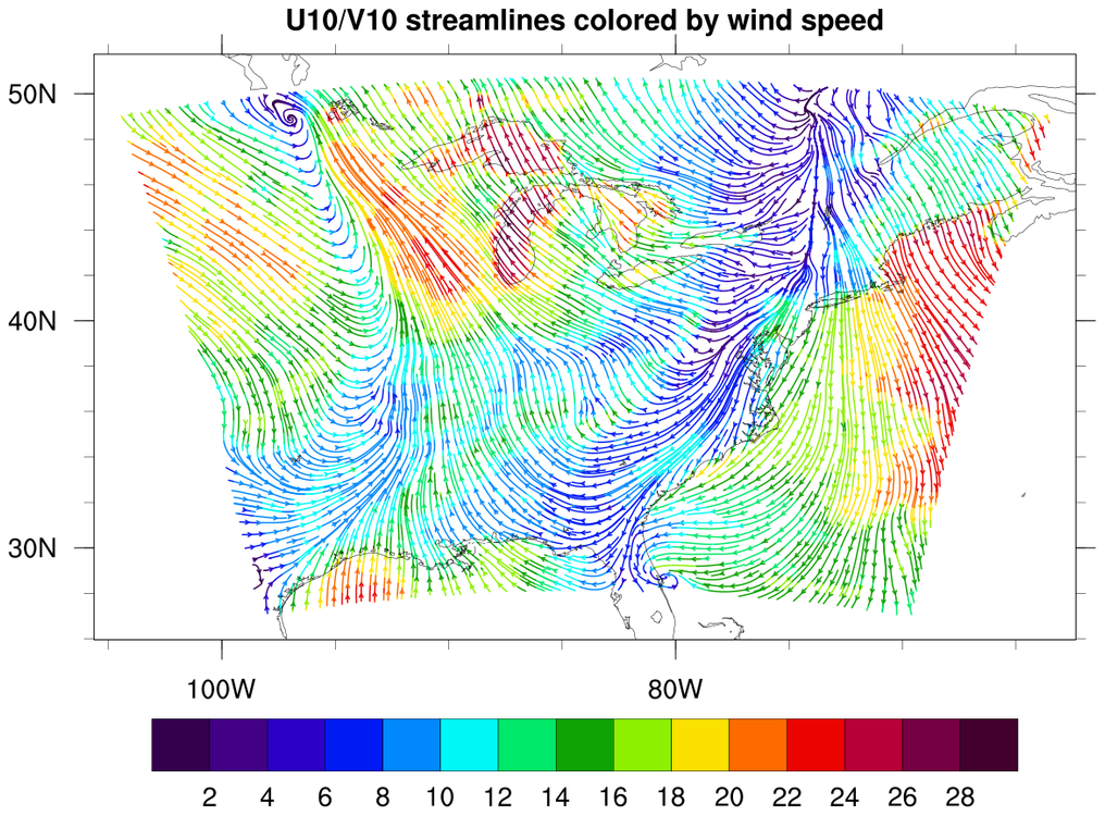
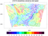
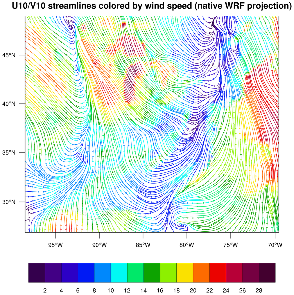
wrf_gsn_8.ncl This example shows how to generate streamlines of U10/V10, colored by wind speed. It uses the gsn_csm_streamline_scalar_map function, which was added in NCL Version 6.3.0.

The first plot shows the streamlines drawn in a basic lat/lon projection, by reading the XLAT/XLONG data off the WRF output file and attaching them as special "lat2d" and "lon2d" attributes to the data being plotted.

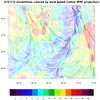
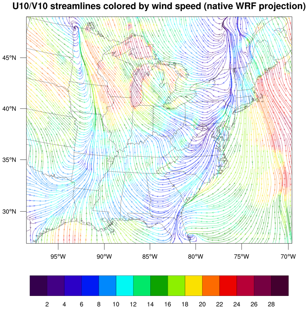
The second plot shows the same streamlines drawn in the native WRF map projection. It uses wrf_map_resources to set the correct map resources. Note that the special resource tfDoNDCOverlay needs to be set to True to tell NCL that the data is being plotted in a native projection.

In the second plot, it's hard to see the map outlines. The third plot shows how to set map resources to thicken the map outlines and to make the streamlines less vivid.

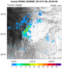
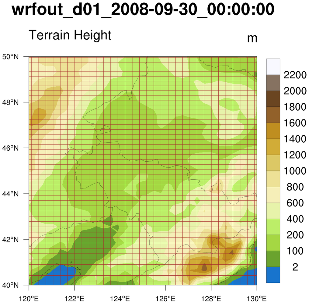
animate_4_1.ncl /
animate_4_2.ncl:

This example shows two ways to create a 97-frame 4-panel animation in NCL, with tips on how to speed things up.

The animation is filled contours of WRF reflectivity (across time and four selected level indexes) overlaid on a WRF terrain plot. The terrain plot is the same for each iteration, while the reflectivity plots change for each time and level.

animate_4_1.ncl - this script shows the traditional and "easy" way to do this, but also potentially slower, by calling gsn_csm_contour, gsn_csm_contour_map, and overlay each time in the loop.

animate_4_2.ncl - this script shows how to speed this up a little by using "setvalues" on existing reflectivity plots to simply change the data.

The timings on a Mac system were as follows:

"animate_4_1.ncl" - 163.0 seconds
"animate_4_2.ncl" - 129.8 seconds

Click on thumbnail image for an animation

The animation was created by generating a series of PNG images, and then calling:

convert animate*.00*png animate_4.gif

wrf_gsn_9.ncl This example plots WRF data over the France/Spain region, and compares map resolutions from:

• NCL's "MediumRes" map outlines
• RANGS database high-res coastal outlines
• shapefile outlines

Instructions for getting the RANGS database can be found at: http://www.ncl.ucar.edu/Document/Graphics/rangs.shtml

The shapefile outlines for France and Spain were downloaded from http://www.gadm.org/country

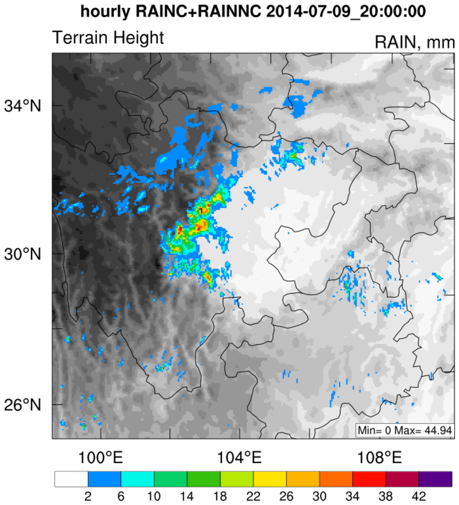
WRF_pcp_2.ncl: This example shows how to overlay precipitation contours on a grayscale terrain map, using transparency to control the colors for precipitation.

gsn_csm_contour_map is used to create the base terrain plot, and gsn_csm_contour is used for the precipitation plot. wrf_map_resources is used to get the correct map projection parameters as defined on the WRF file.

This script was contributed by Xiao-Ming Hu (xhu@ou.edu) at the Center for Analysis and Prediction of Storms, University of Oklahoma.

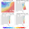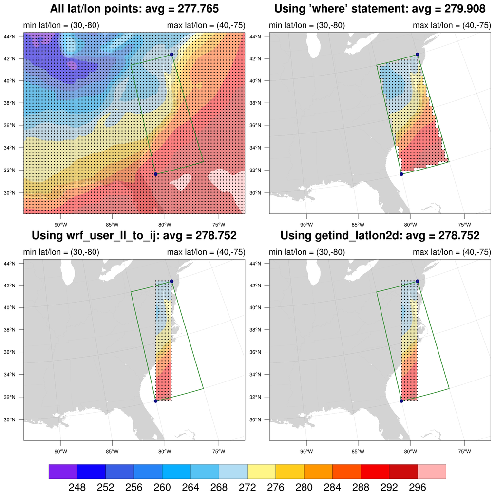
wrf_gsn_10.ncl This example shows three ways to subset a WRF lat/lon grid by providing two corners of a lat/lon box. Using each method, a spatial average is taken of the data in this box.

The three methods are 1) where, 2) wrf_user_ll_to_xy, 3) getind_latlon2d.

Markers are drawn in the plots to show the area where the data was subsetted, so you can see there is quite a difference in the two methods.

wrf_user_ll_to_xy should only be used on WRF-ARW data. The other methods will work on curvilinear grids.

This example was based on wrf_debug_4.ncl.