NCL Home > Documentation > Functions > CESM

albedo_ccm

Computes albedo via CESM model radiation variables.

Available in version 6.4.0 and later.

Prototype

load "$NCARG_ROOT/lib/ncarg/nclscripts/csm/contributed.ncl"  ; This library is automatically loaded
                                                             ; from NCL V6.2.0 onward.
                                                             ; No need for user to explicitly load.

	function albedo_ccm (
		flux1       : numeric,  
		flux2       : numeric,  
		formula [1] : integer   
	)

	return_val [dimsizes(flux)] :  float or double

Return value

An array of the same size, shape and type as flux1.

Description

A simple albedo calculuation which uses:

     albedo = (flux1-flux2)/flux1     ; formula=0
or
     albedo =  flux2/flux1            ; formula=1

Where flux1=0.0, the returned value is set to _FillValue.

While originally written and tested for CAM variables, this function can be used with any appropriate radiation variables. For example, the CLM output data includes several spectral fluxes. See examples.

Because the albedo is a ratio, using monthly mean radiation values would (likely) not yield the same result as computing the monthly mean values from the (say) hourly or daily mean albedos. Still, the result could be useful.

Examples

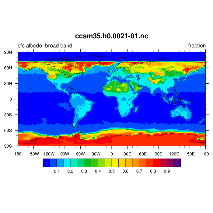
Example 1: CAM file(s). For multiple files use addfiles, fsds=fccm[:]->FSDS and fsns=fclm[:]->FSNS


     filc  = "ccsm35.h0.0021-01.nc"
     fccm  = addfile (filc , "r")   ; January monthly file
     fsds  = fccm->FSDS                   
     fsns  = fccm->FSNS

     alb_0 = albedo_ccm(fsds, fsns, 0)    ; 0 => (flux1-flux2)/flux1  =>(fsds-fsns)/fsds 

     alb_0@long_name = "sfc albedo: broad band"  ; (optional) replace generic long_name
     printVarSummary(alb_0) 
     print("alb_0: min="+min(alb_0)+"  max="+max(alb_0))

     wks   = gsn_open_wks ("png", "albedo" ) ; open workstation 
     gsn_define_colormap(wks, "BlAqGrYeOrReVi200")
     res                      = True                    
     res@cnFillOn             = True
     res@cnLinesOn            = False
     res@cnLineLabelsOn       = False
     res@cnLevelSelectionMode = "ManualLevels"  ; set manual contour levels
     res@cnMinLevelValF       =  0.05           ; set min contour level
     res@cnMaxLevelValF       =  0.95           ; set max contour level
     res@cnLevelSpacingF      =   .05           ; set contour spacing
     res@tiMainString         = filc
   
     plot = gsn_csm_contour_map(wks,alb_0(0,:,:), res)

A sample printVarSummary output follows. The sample graphic is here.

     Variable: alb_0
     Type: float
     Total Size: 55296 bytes
                 13824 values
     Number of Dimensions: 3
     Dimensions and sizes:	[time | 1] x [lat | 96] x [lon | 144]
     Coordinates: 
                 time: [7331..7331]
                 lat: [ -90..89.99999999999999]
                 lon: [   0..357.5]
     Number Of Attributes: 4
       _FillValue :	1e+10
       long_name :	sfc albedo: broad band       <= generic long_name is 'albedo'
       units :	fraction
       formula :         formula=0:       albedo = (flux1-flux2)/flux1

     (0)	albedo: min=0  max=0.851161

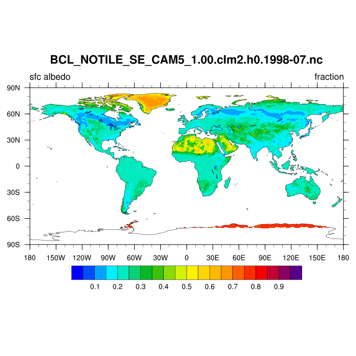
Example 2: CLM file(s). For multiple files use addfiles and fsdsnd=fclm[:]->FSDSND and fsrnd=fclm[:]->FSRND


     filc   = "CLM.1998-07.nc"
     fclm   = addfile (filc , "r")            ; July monthly file
     fsdsnd = fclm->FSDSND         ; flux1; (time,ncells)
     fsrnd  = fclm->FSRND          ; flux2                 
     alb_1  = albedo_ccm(fsdsnd, fsrnd, 1)    ; 1 => flux2/flux1 

     alb_1@long_name = "sfc albedo: nir"      ; (optional) replace generic long_name
     printVarSummary(alb_1) 
     print("alb_1: min="+min(alb_1)+"  max="+max(alb_1))

     wks   = gsn_open_wks ("png", "alb_1" ) ; open workstation 
     gsn_define_colormap(wks, "BlAqGrYeOrReVi200")
     res                      = True                    
     res@cnFillOn             = True
     res@cnLinesOn            = False
     res@cnLineLabelsOn       = False
     res@cnLevelSelectionMode = "ManualLevels"  ; set manual contour levels
     res@cnMinLevelValF       =  0.0            ; set min contour level
     res@cnMaxLevelValF       =  0.95           ; set max contour level
     res@cnLevelSpacingF      =   .05           ; set contour spacing
     res@mpFillOn             = True
     res@mpOceanFillColor     = "white"
     res@mpLandFillColor      = "transparent"
     res@mpFillDrawOrder      = "postdraw"

     res@tiMainString         = filc
     plot = gsn_csm_contour_map(wks,alb_1(0,:), res)