NCL Home >
Training >
Workshops
Scripts used in NCL workshop graphics lecture
These examples show a progression of visualizations from the most basic one with no or minimal resources set, to a more complex visualization with multiple resources set. The scripts are named script1a.ncl, script1b.ncl, script1c.ncl, etc to indicate the progression of examples.Click on any of the thumbnails to see a larger image. You can download the NCL scripts by right-clicking on them and doing a "Save As" or "Download linked file". Some of the data files are available for download here, or they may be available on your student machine in class. See instructor for details.
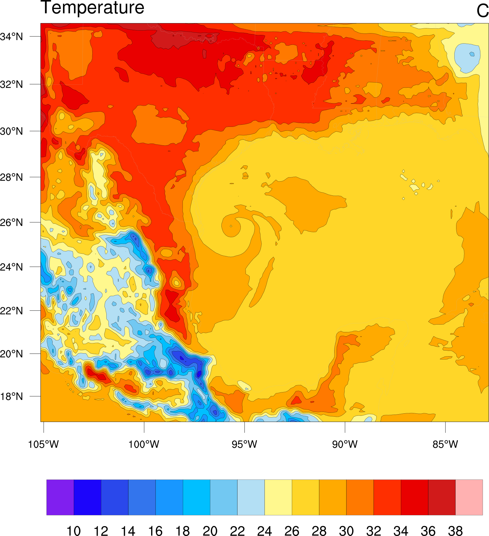
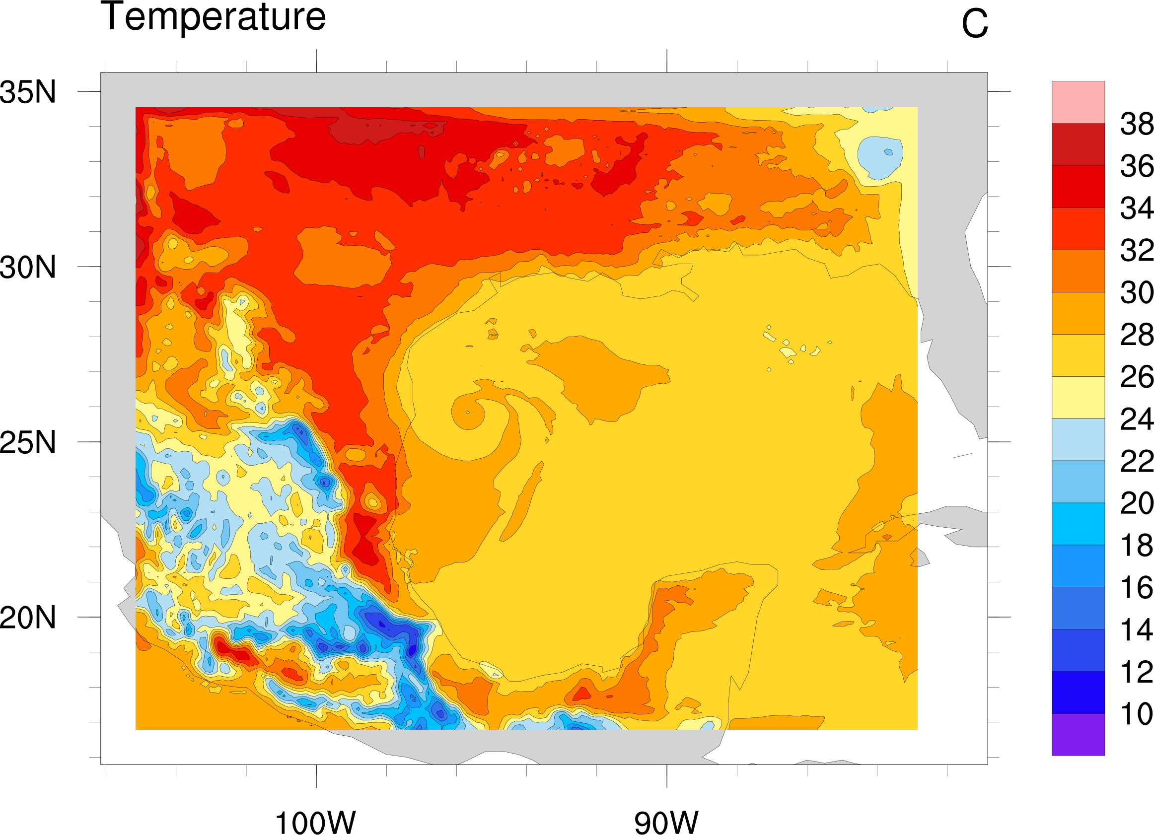
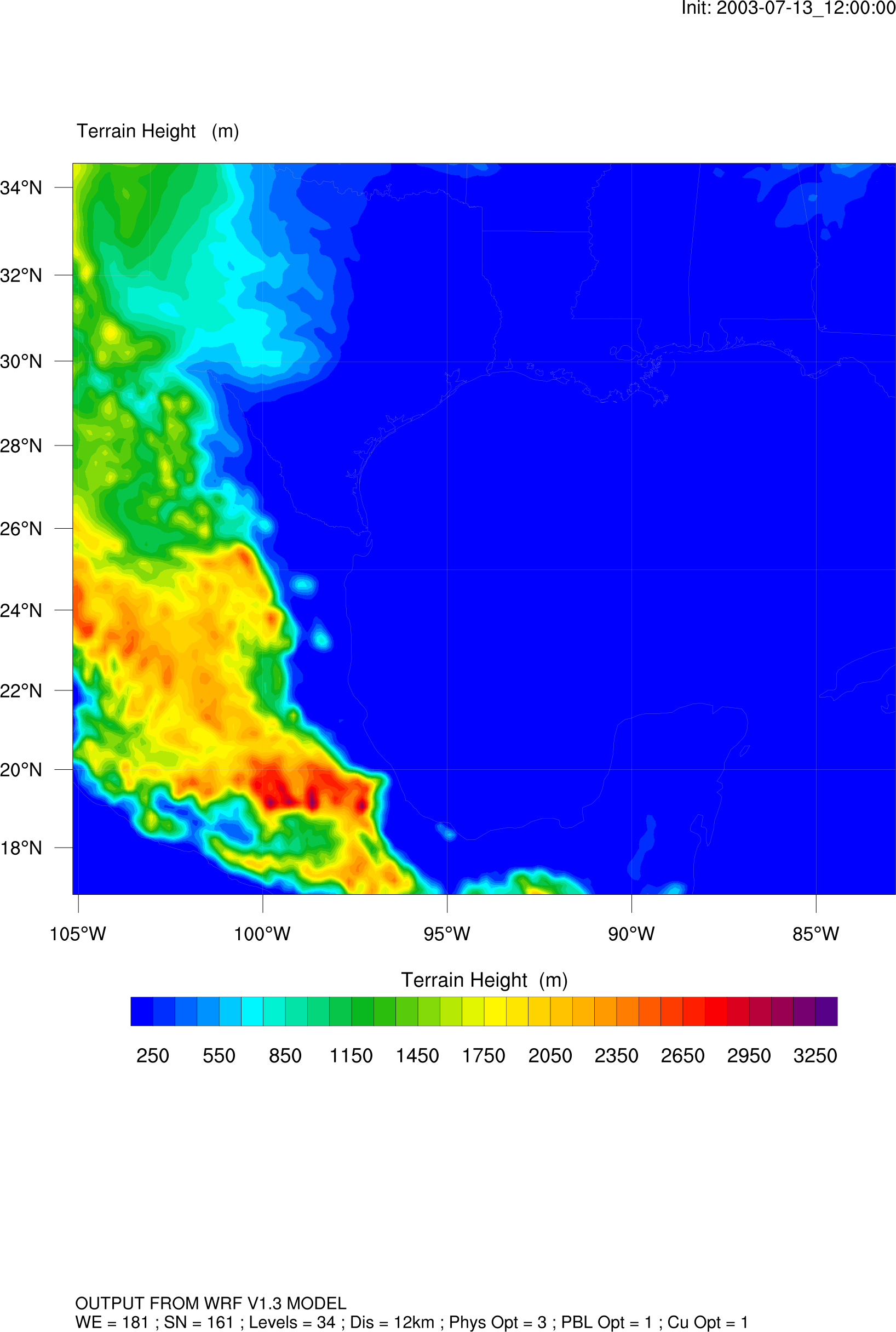
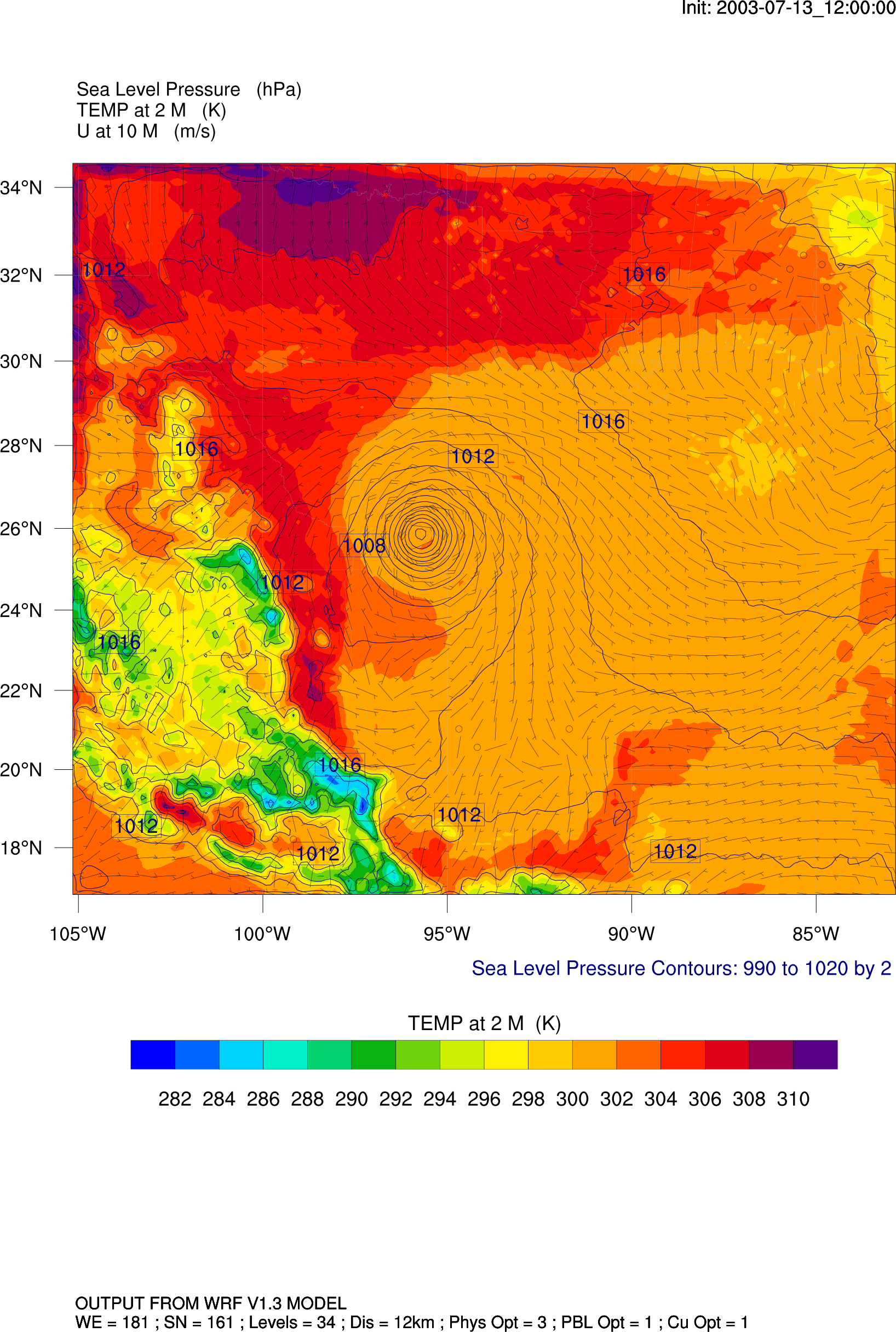
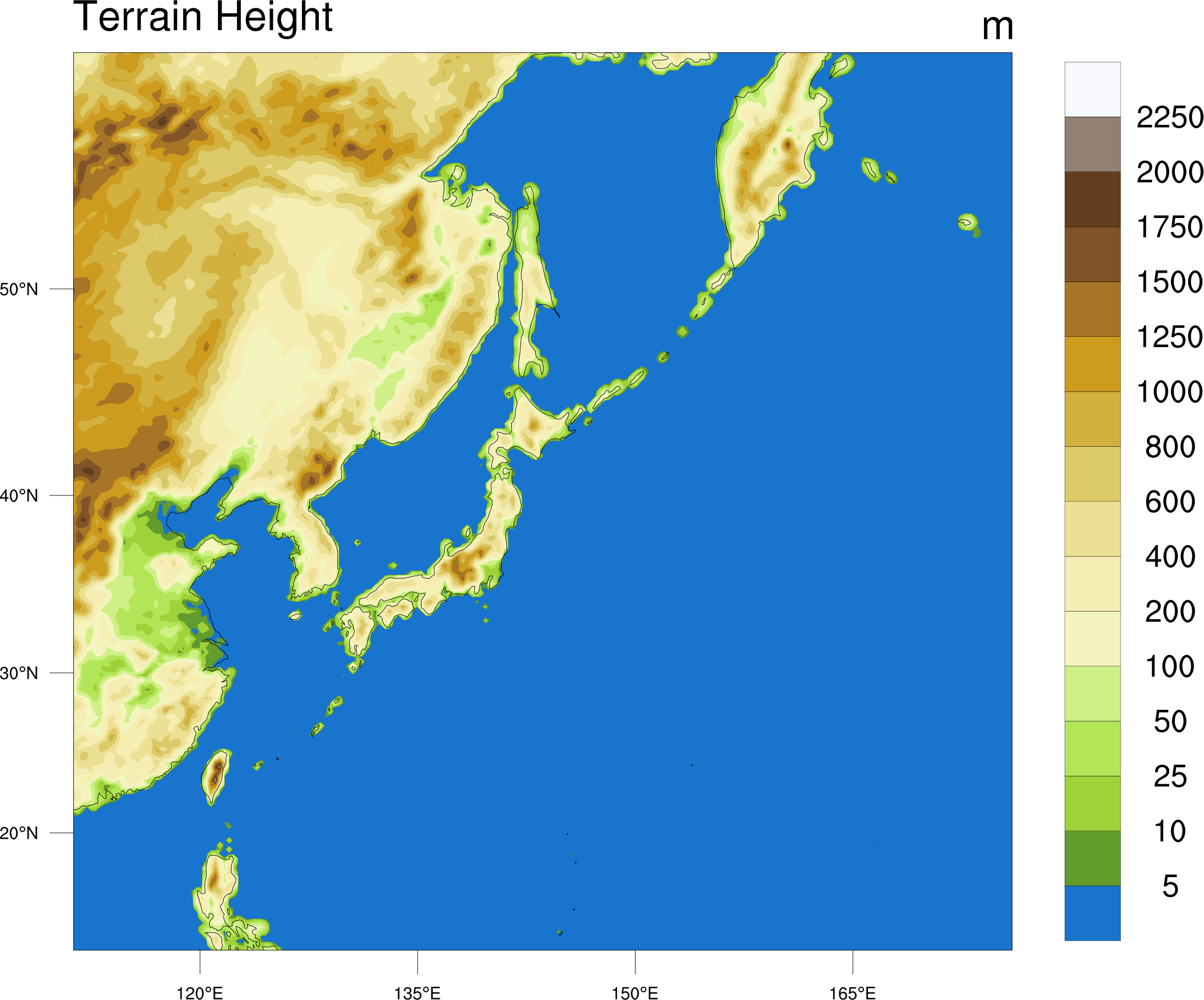
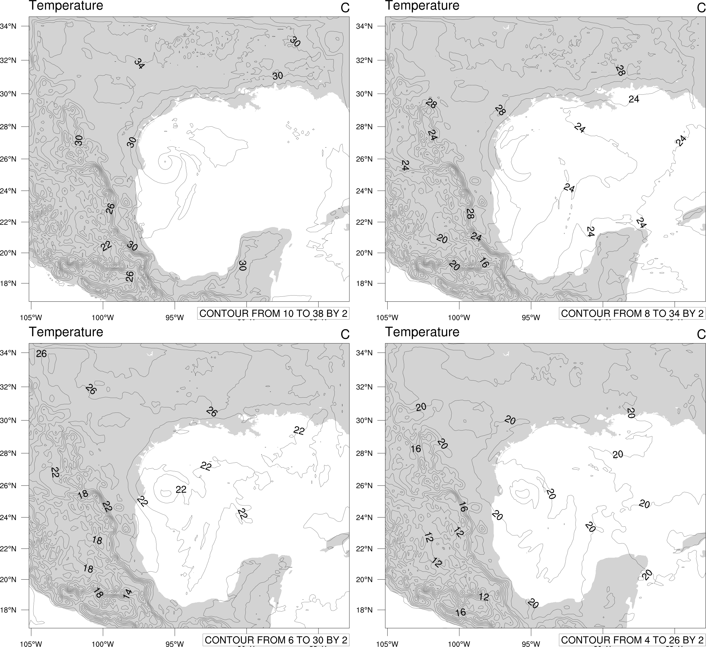
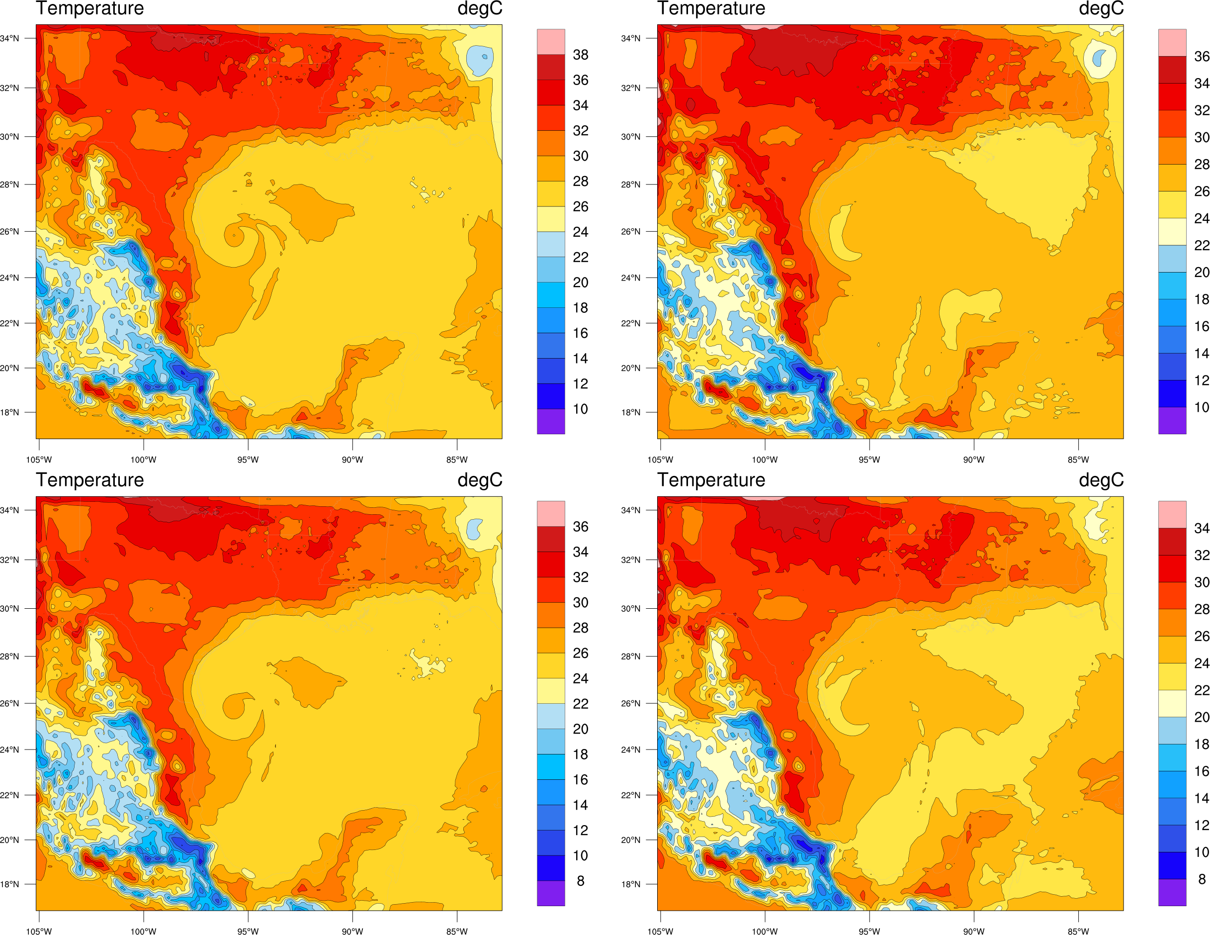
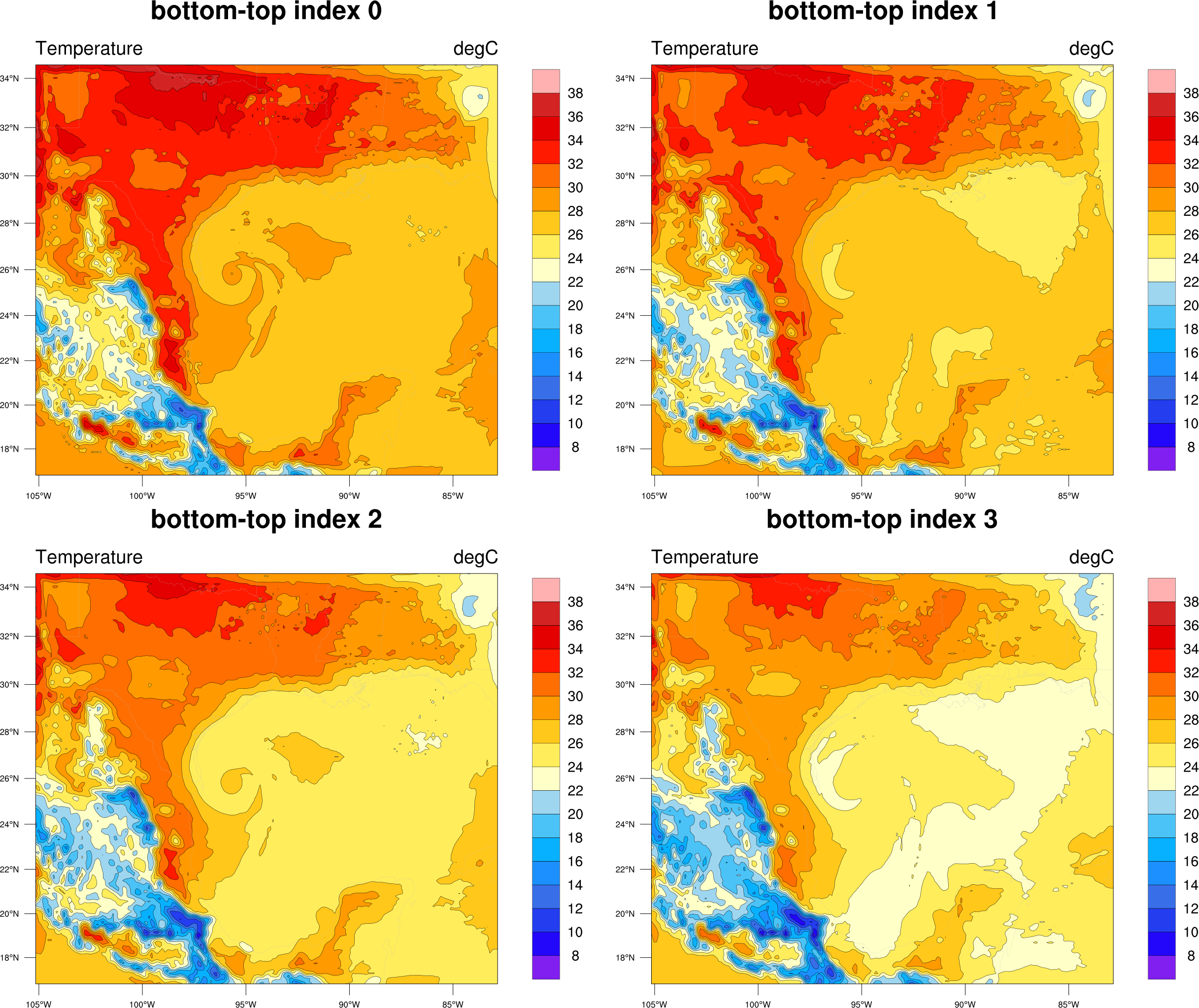
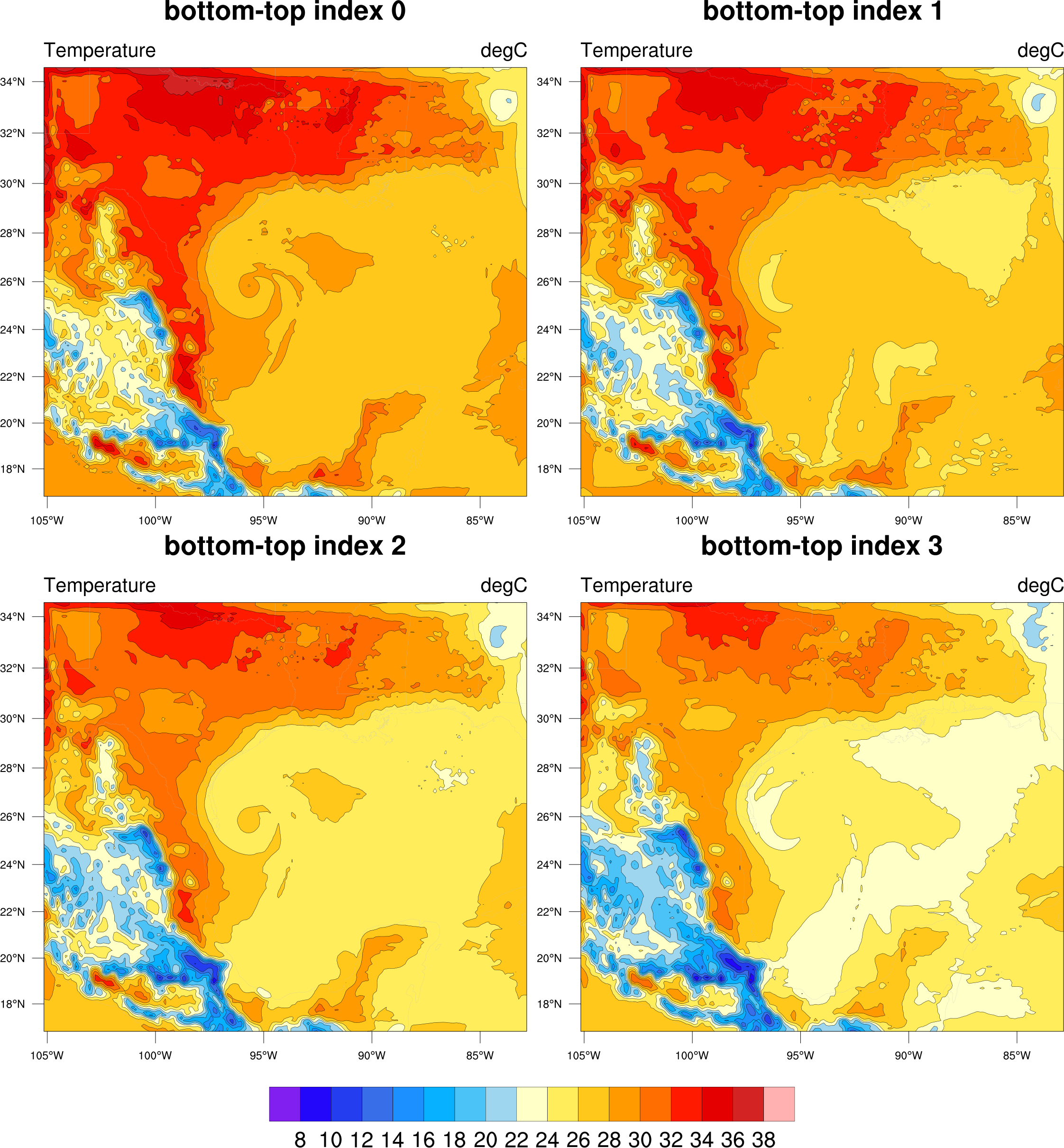
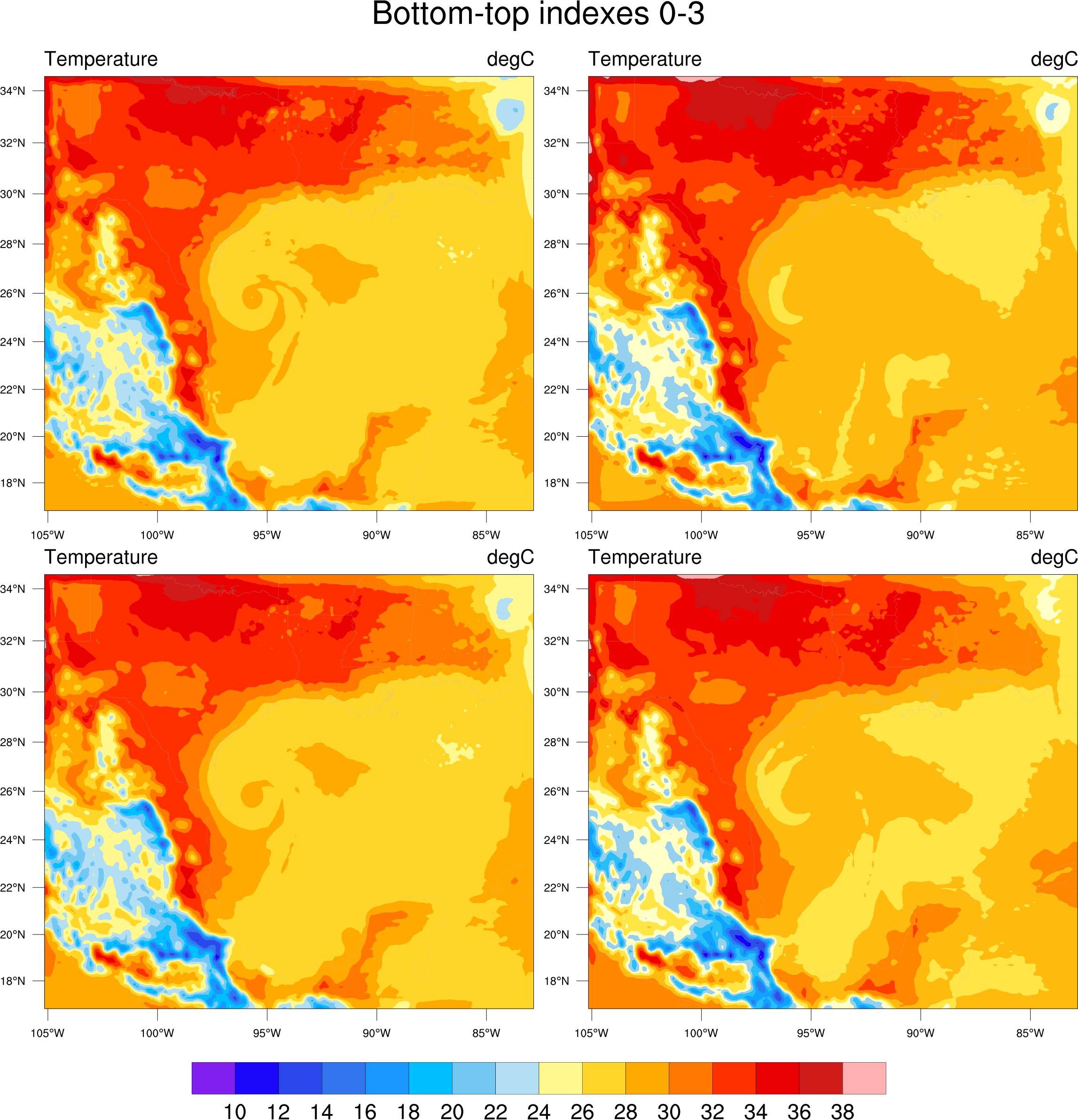
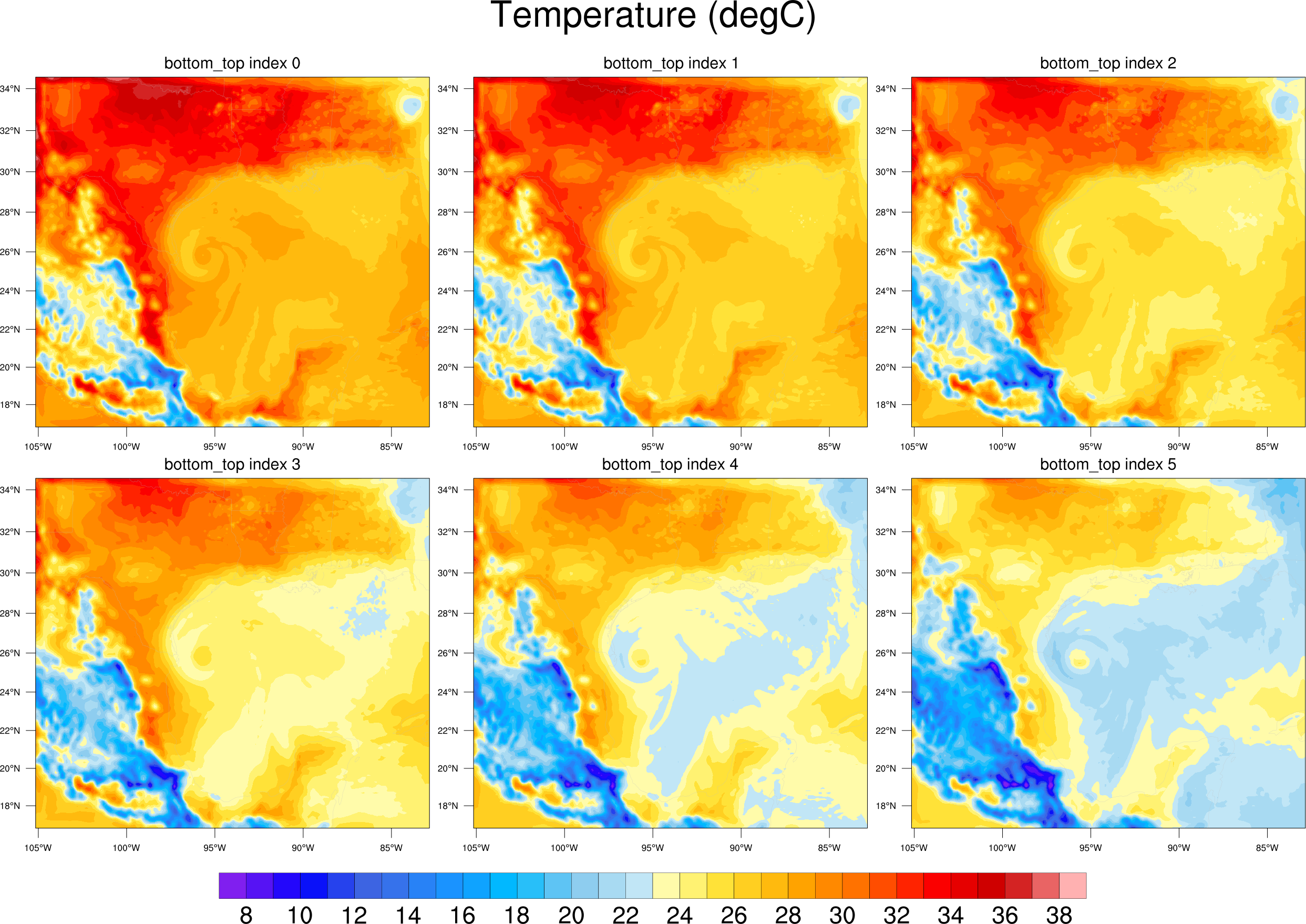
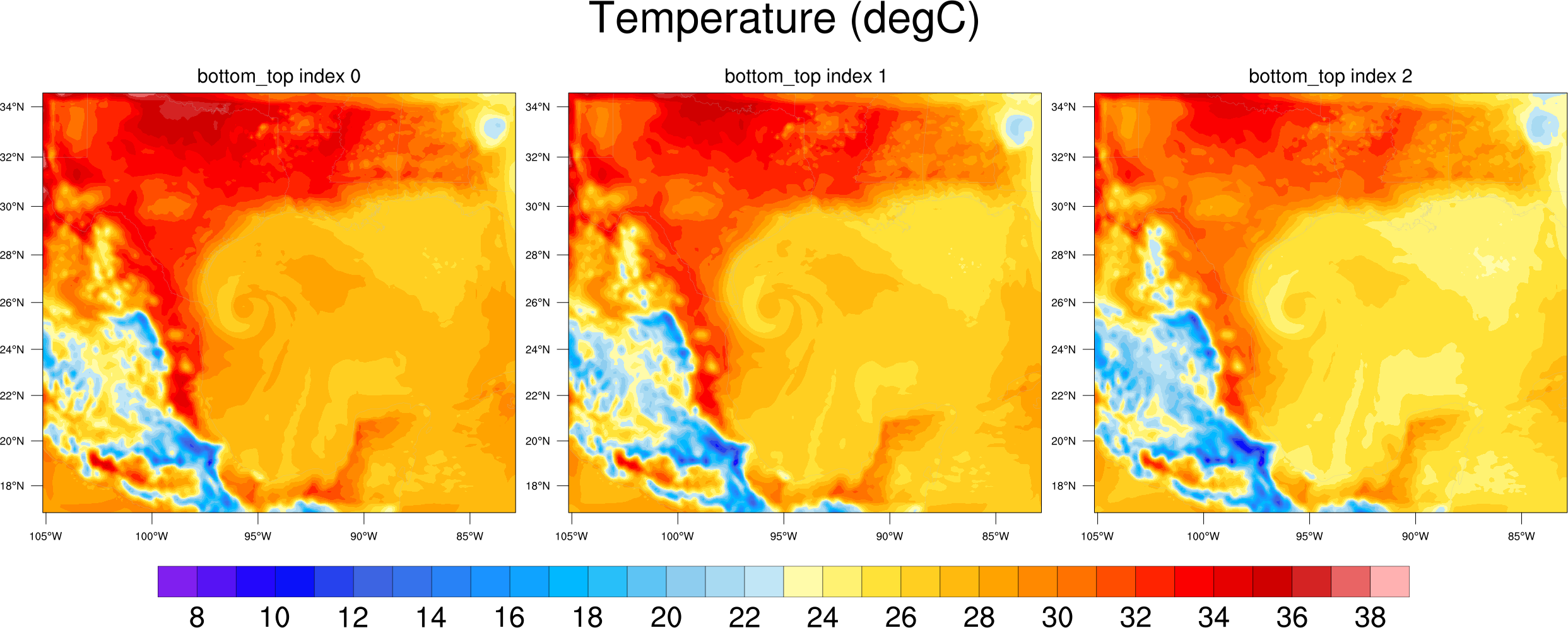
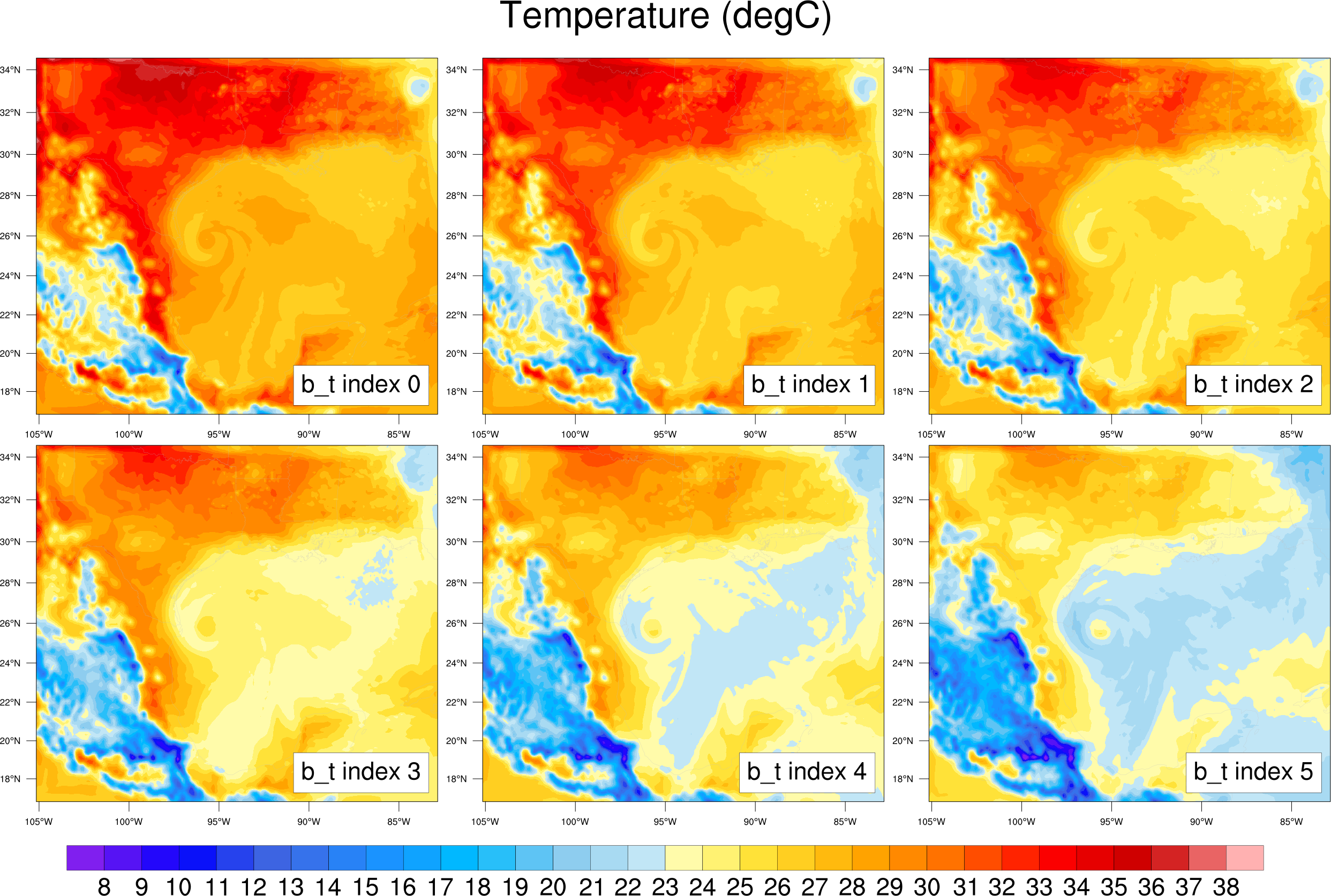
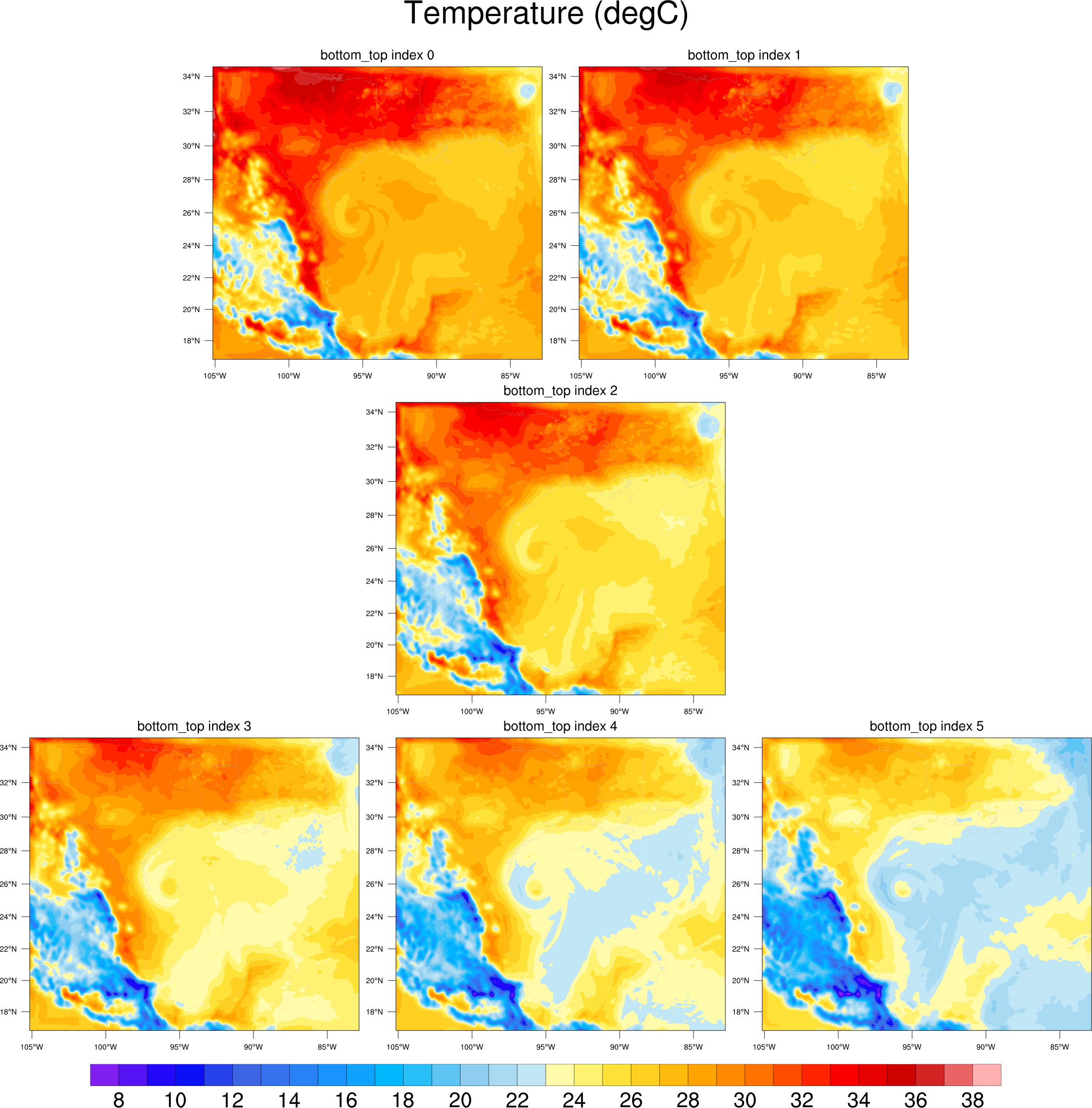
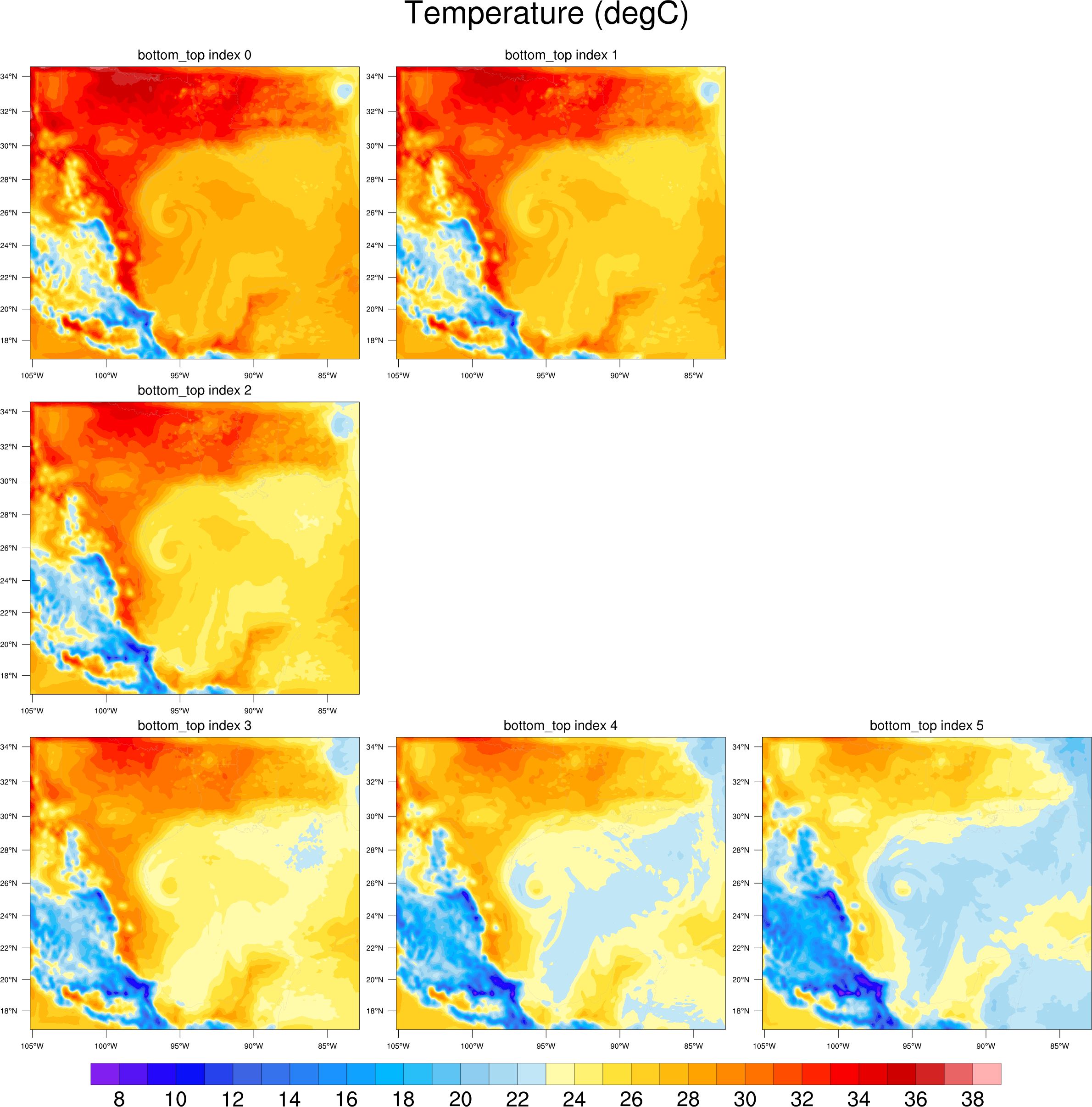
WRF plots

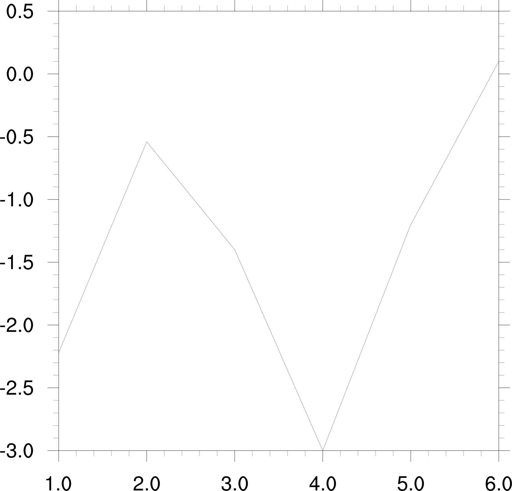
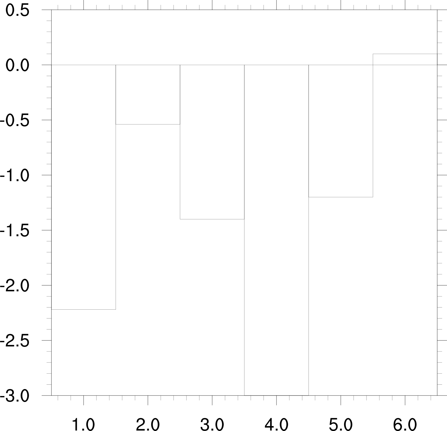
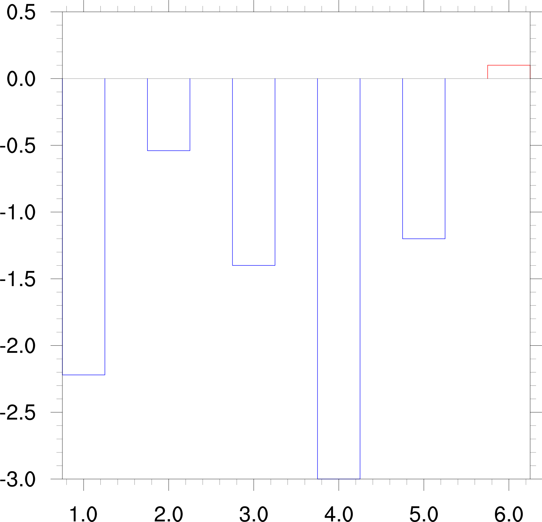
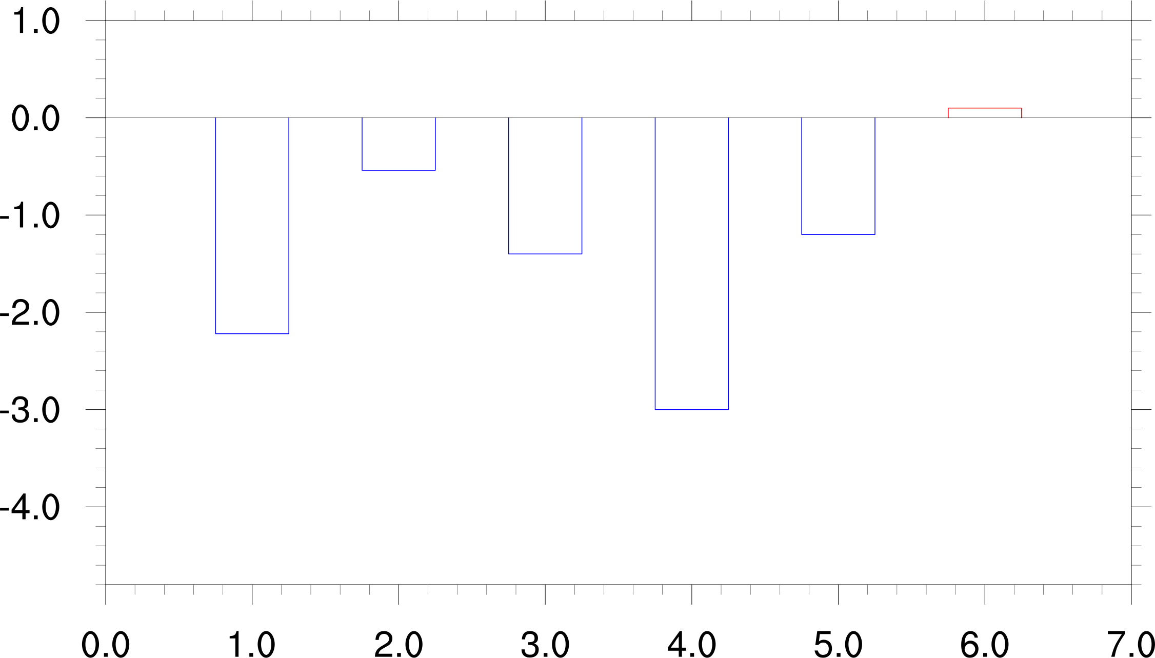
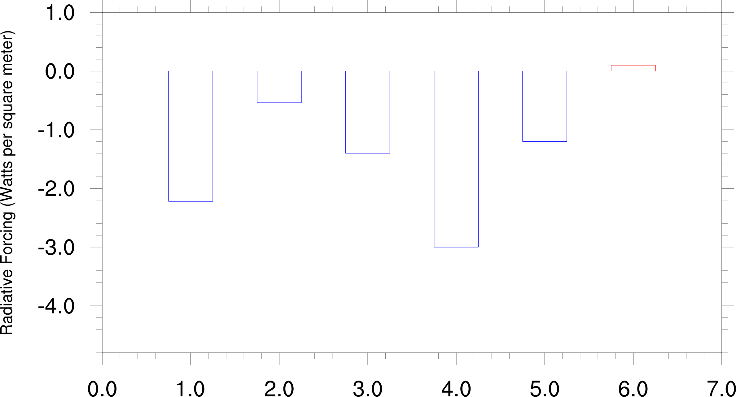
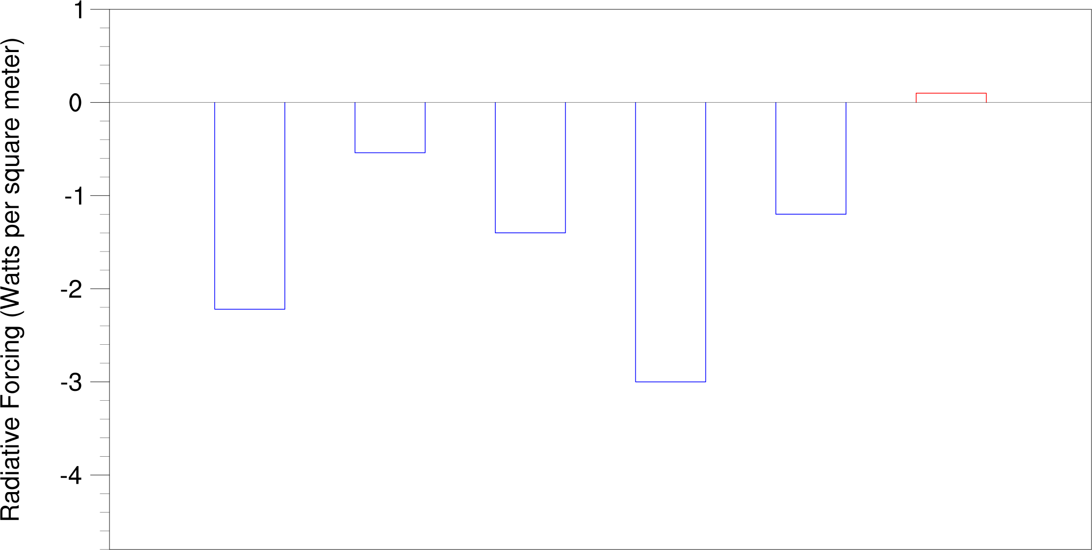
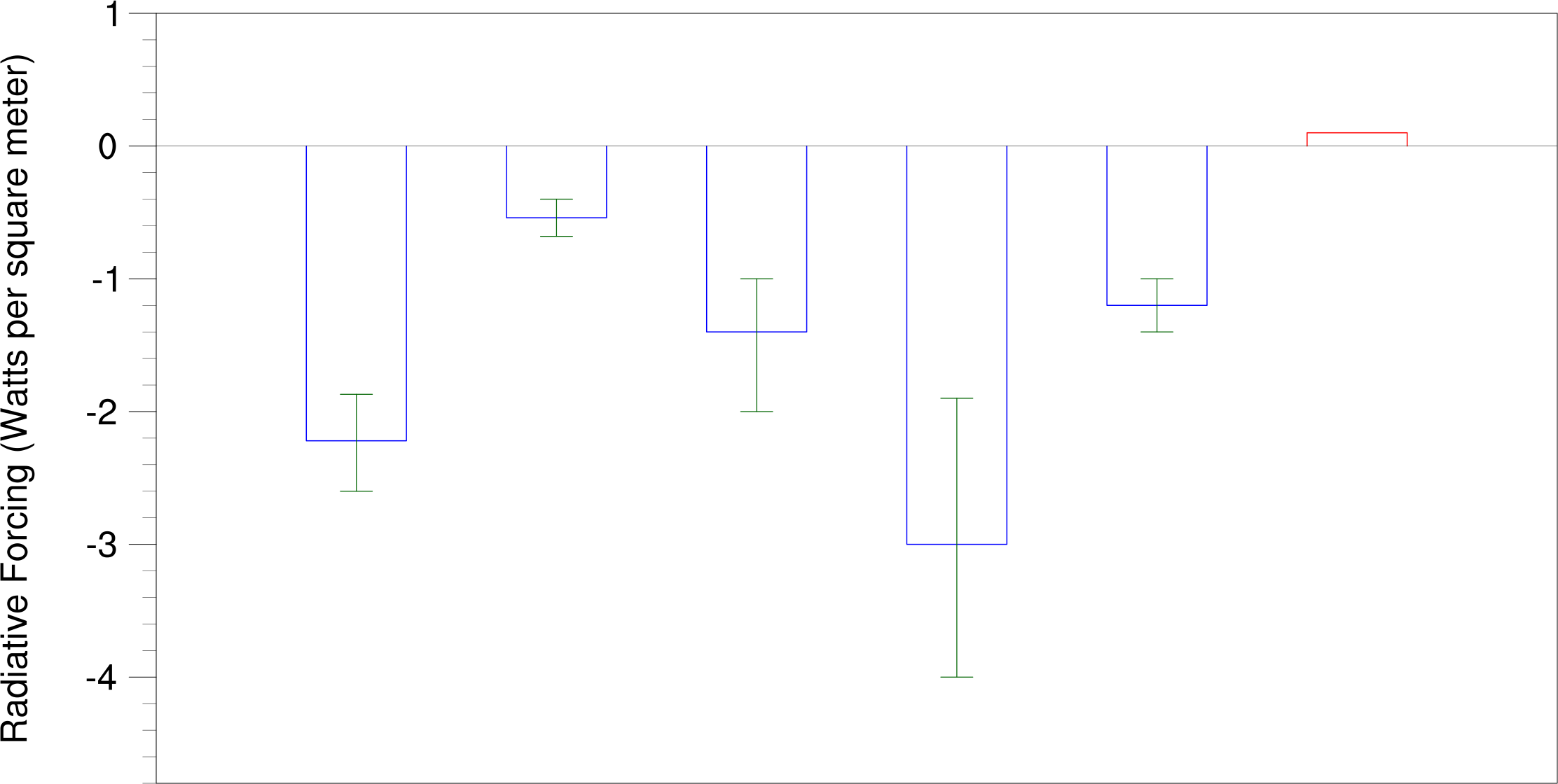
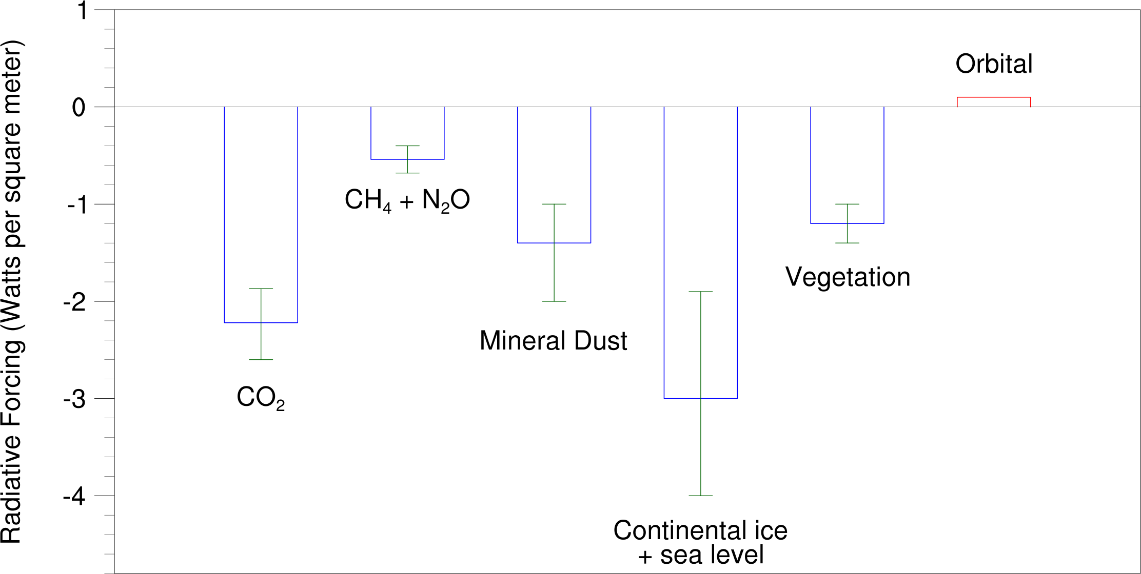
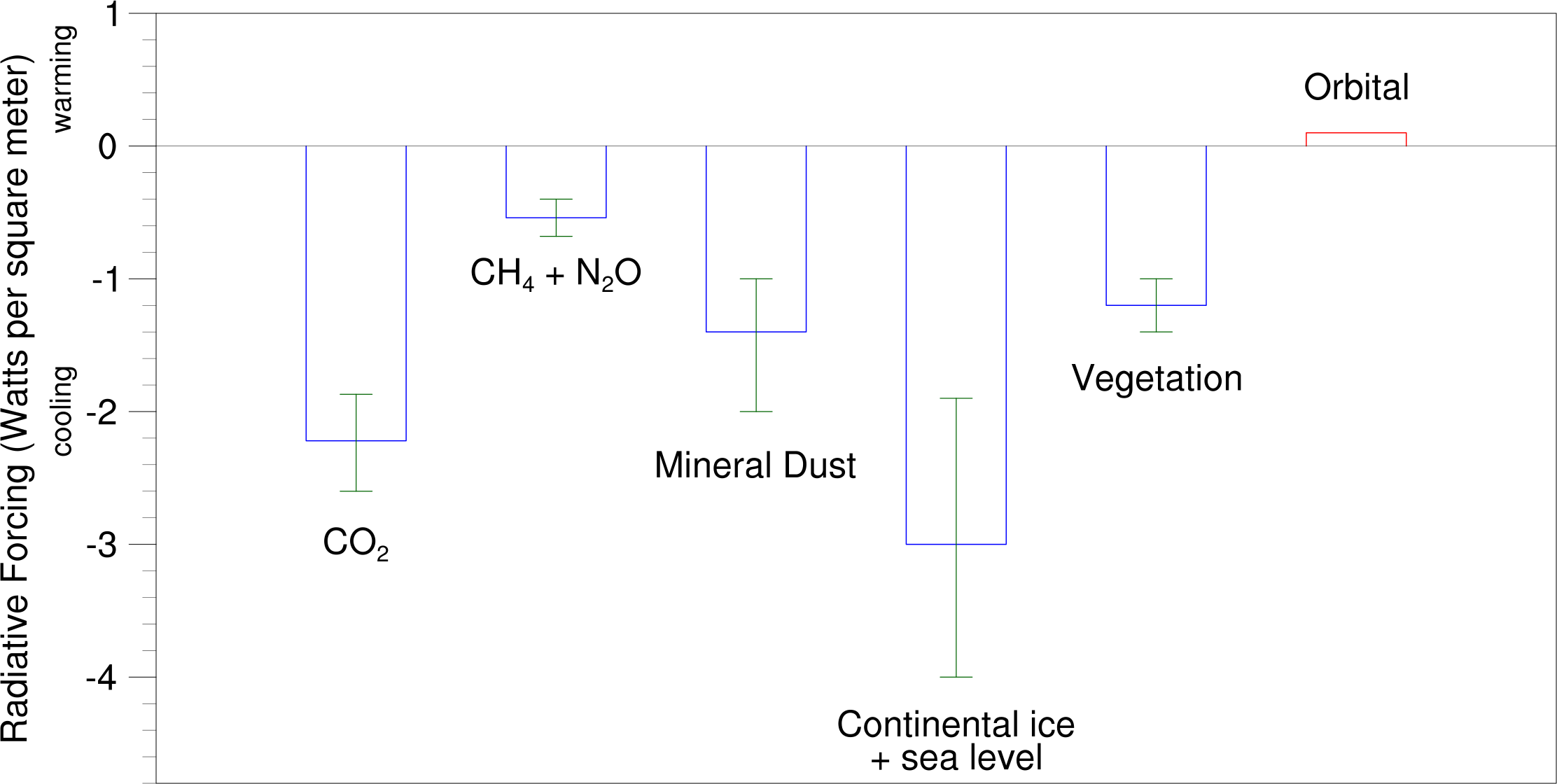
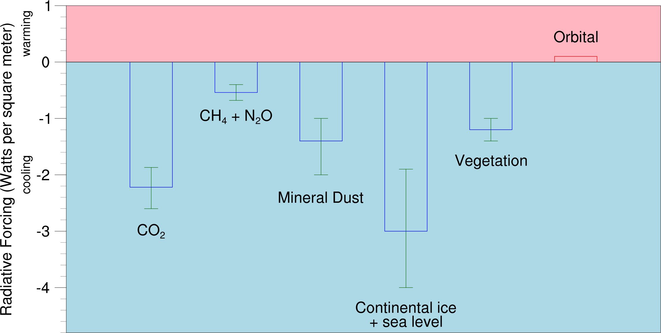
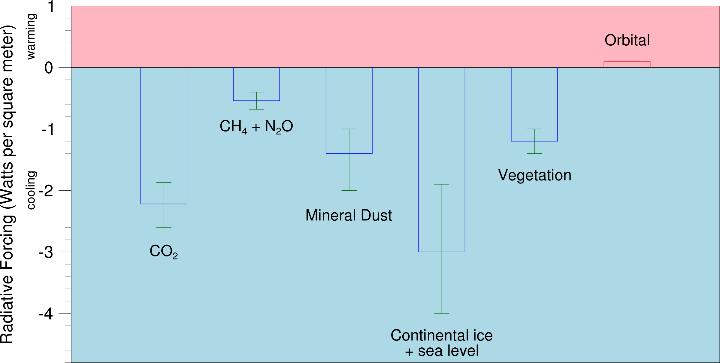
bar charts with primitives
| 
| 
| 
|
| bar1a.ncl | bar1b.ncl | bar1c.ncl | bar1d.ncl |
| 
| 
| 
|
| bar1e.ncl | bar1f.ncl | bar1g.ncl | bar1h.ncl |
| 
| 
| |
| bar1i.ncl | bar1j.ncl | bar1k.ncl |
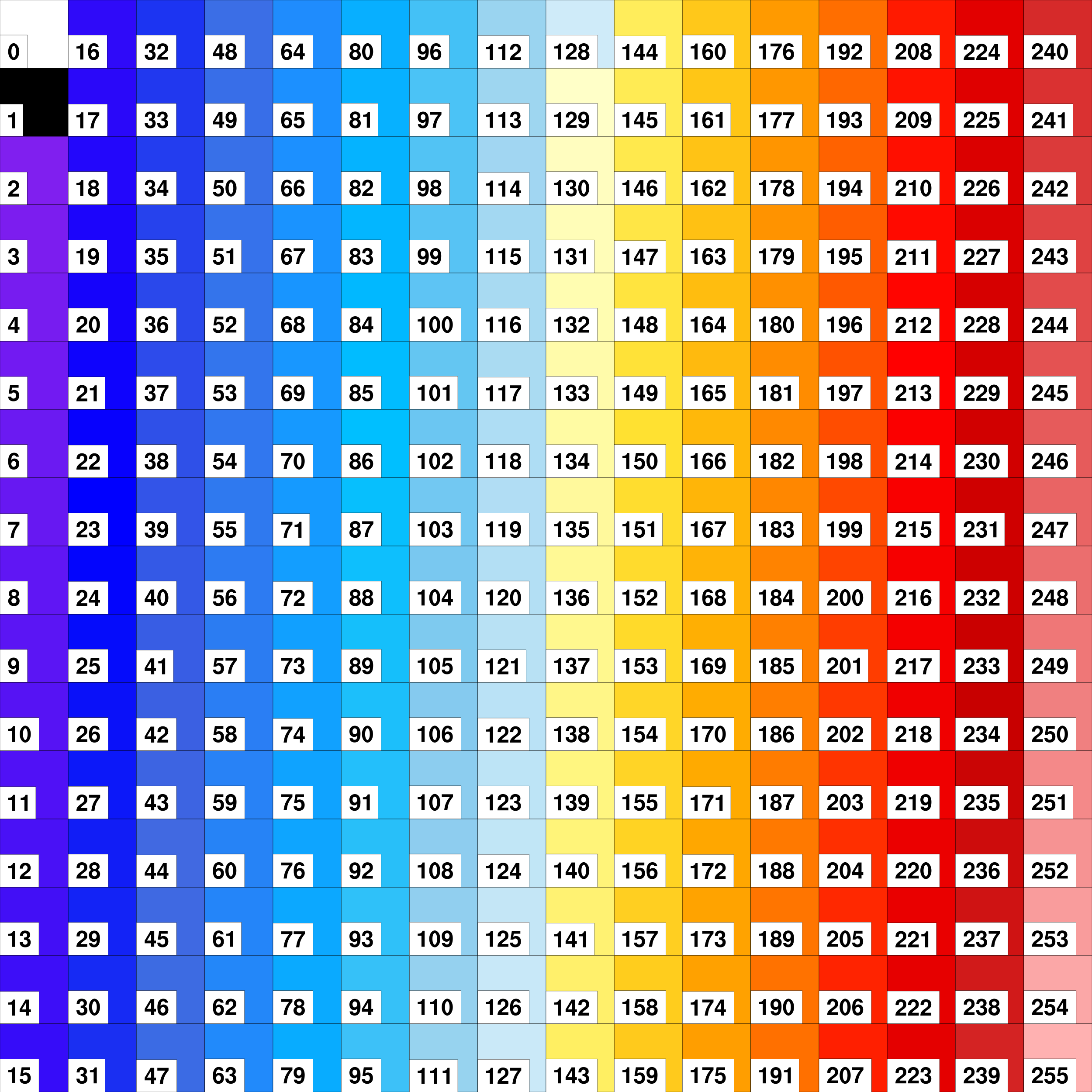
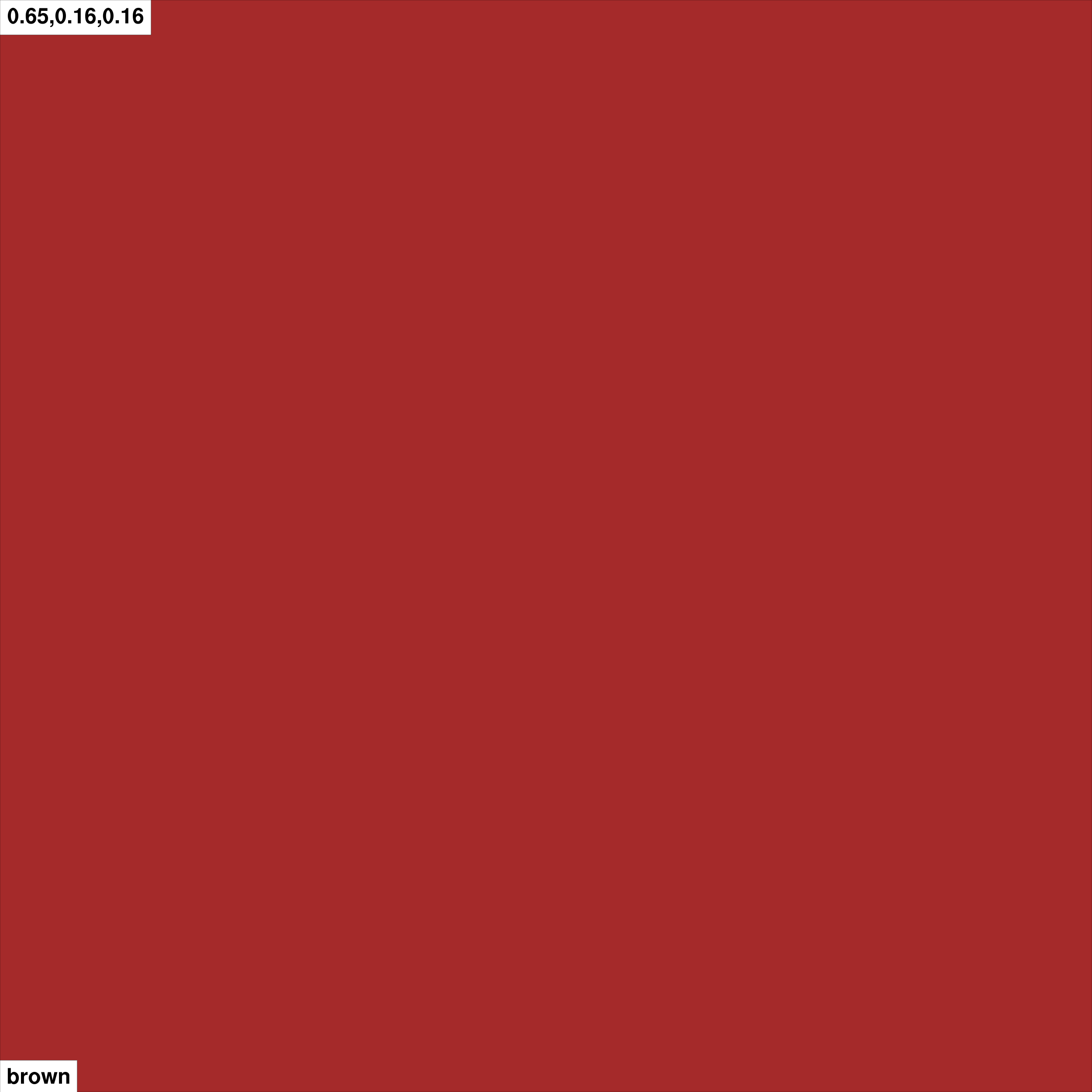
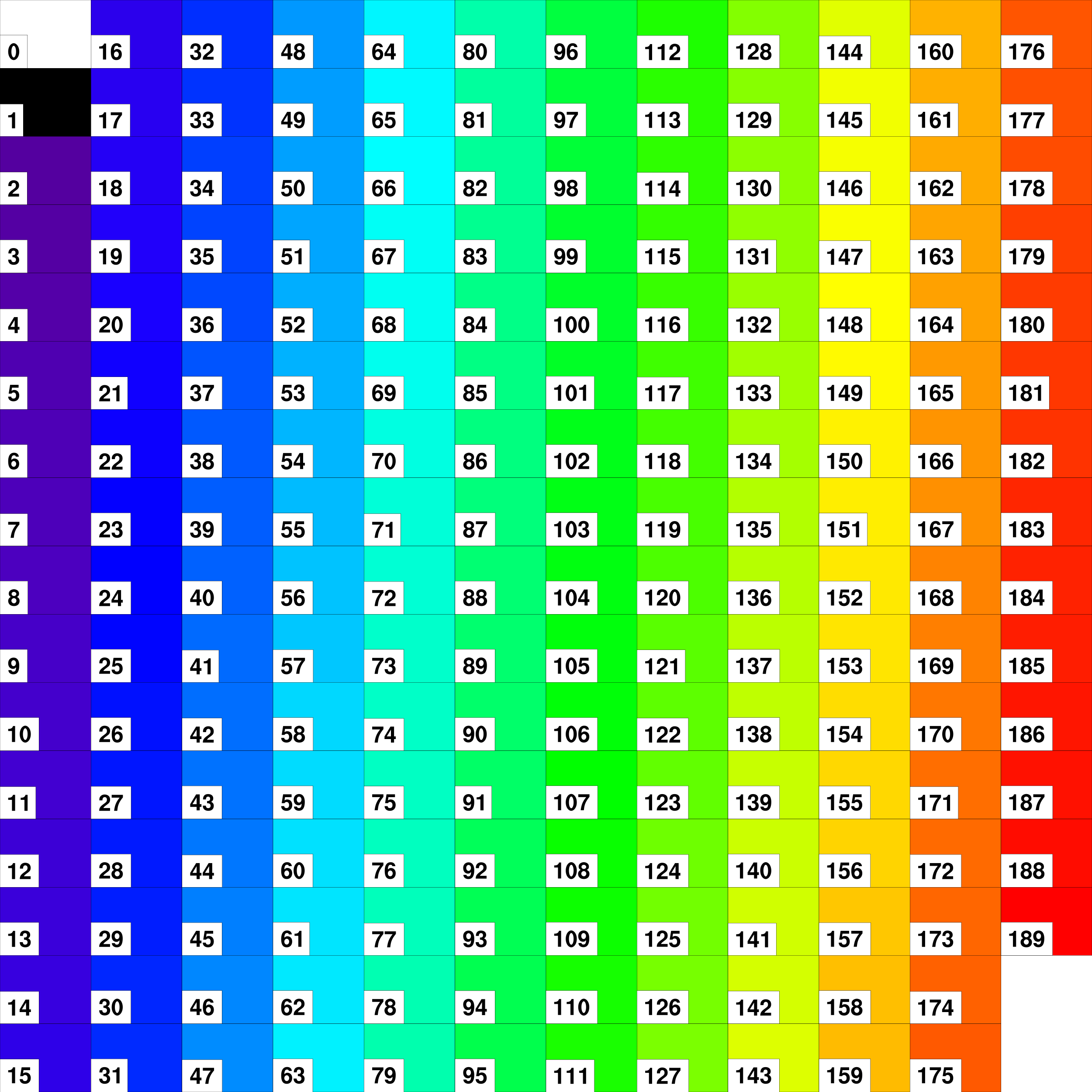
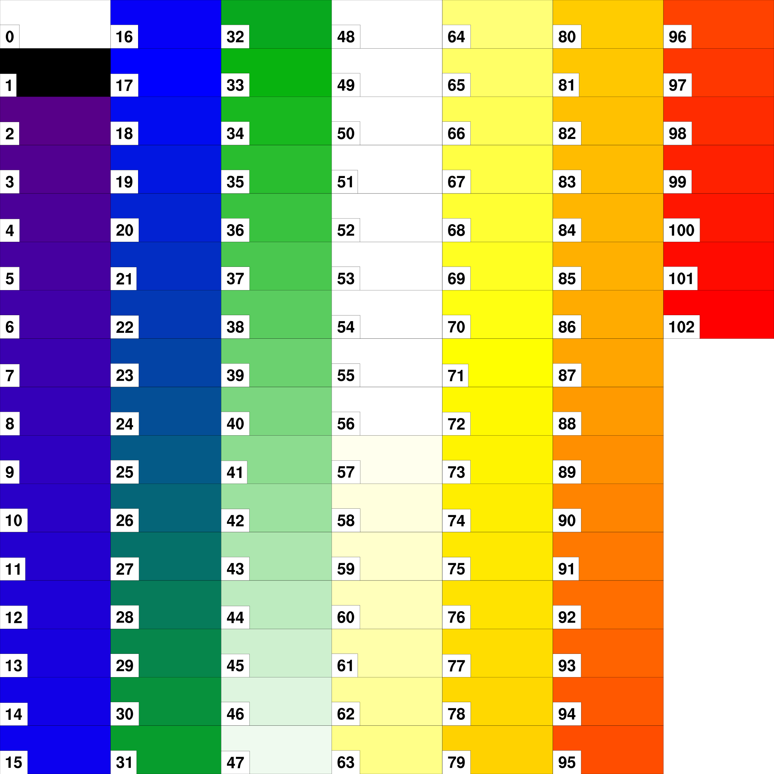
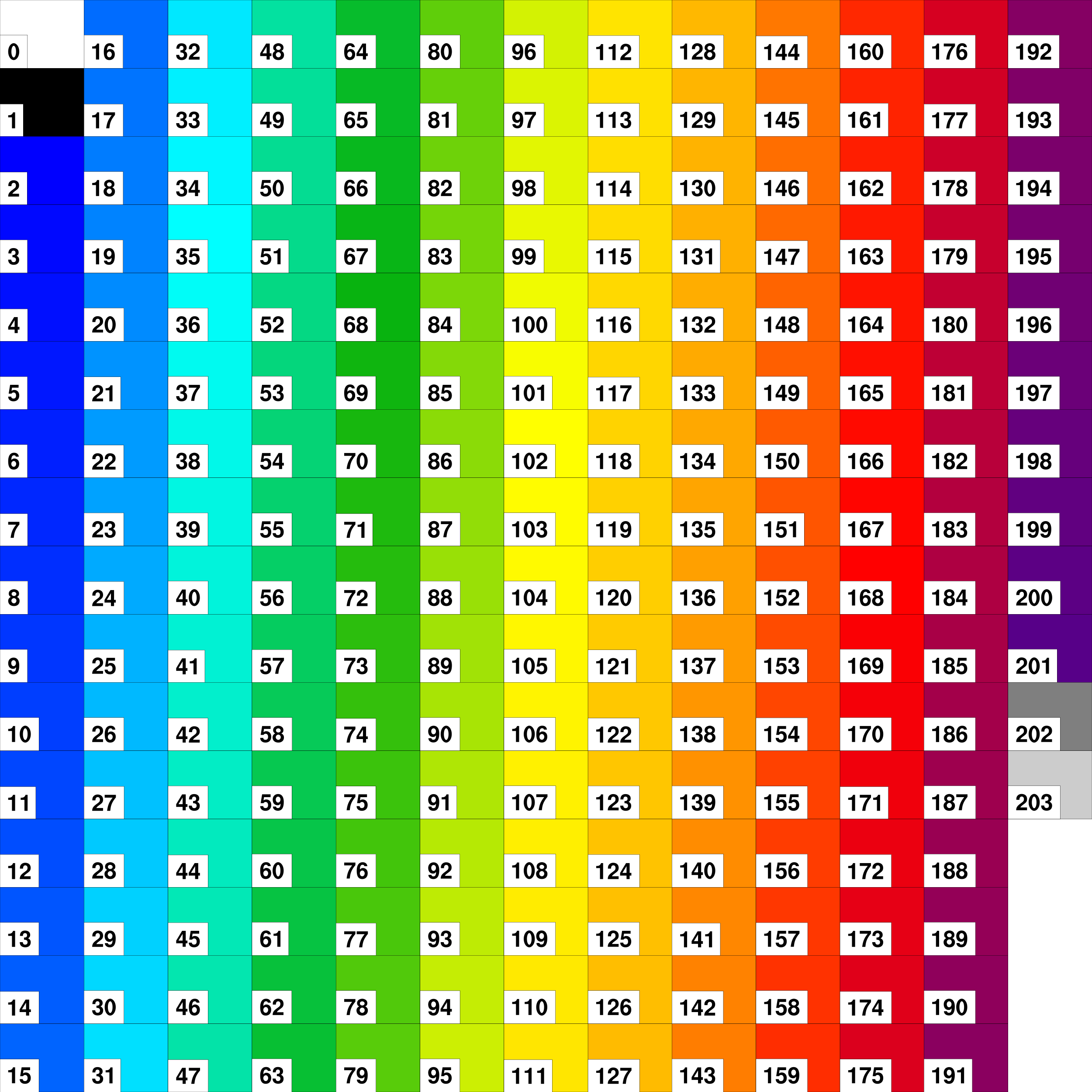
color tables and named colors
| 
| 
| 
|
| color1.ncl | color2.ncl | color3.ncl | color4.ncl |
| 
| 
| |
| color5.ncl | color6.ncl | color7.ncl |
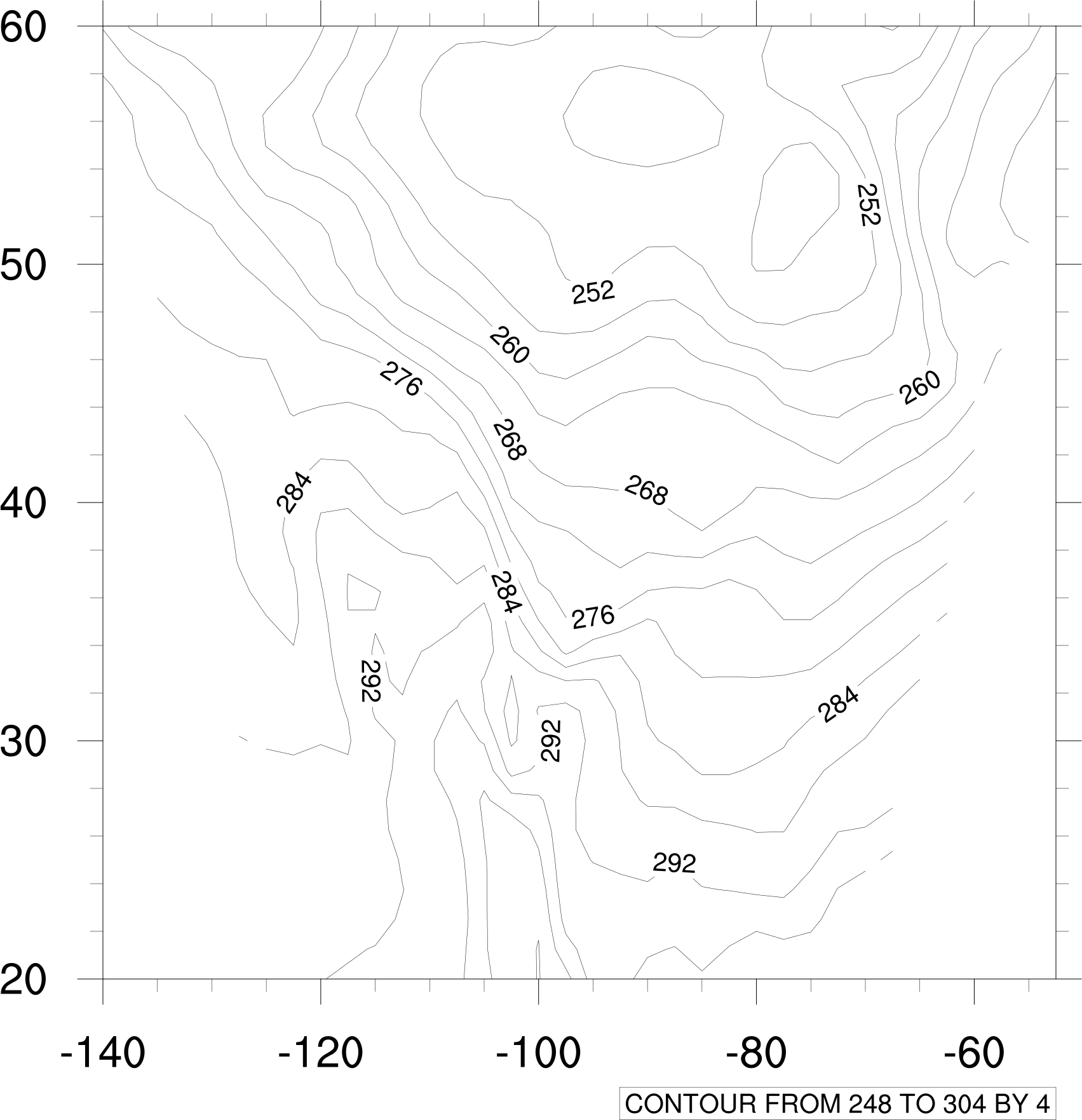
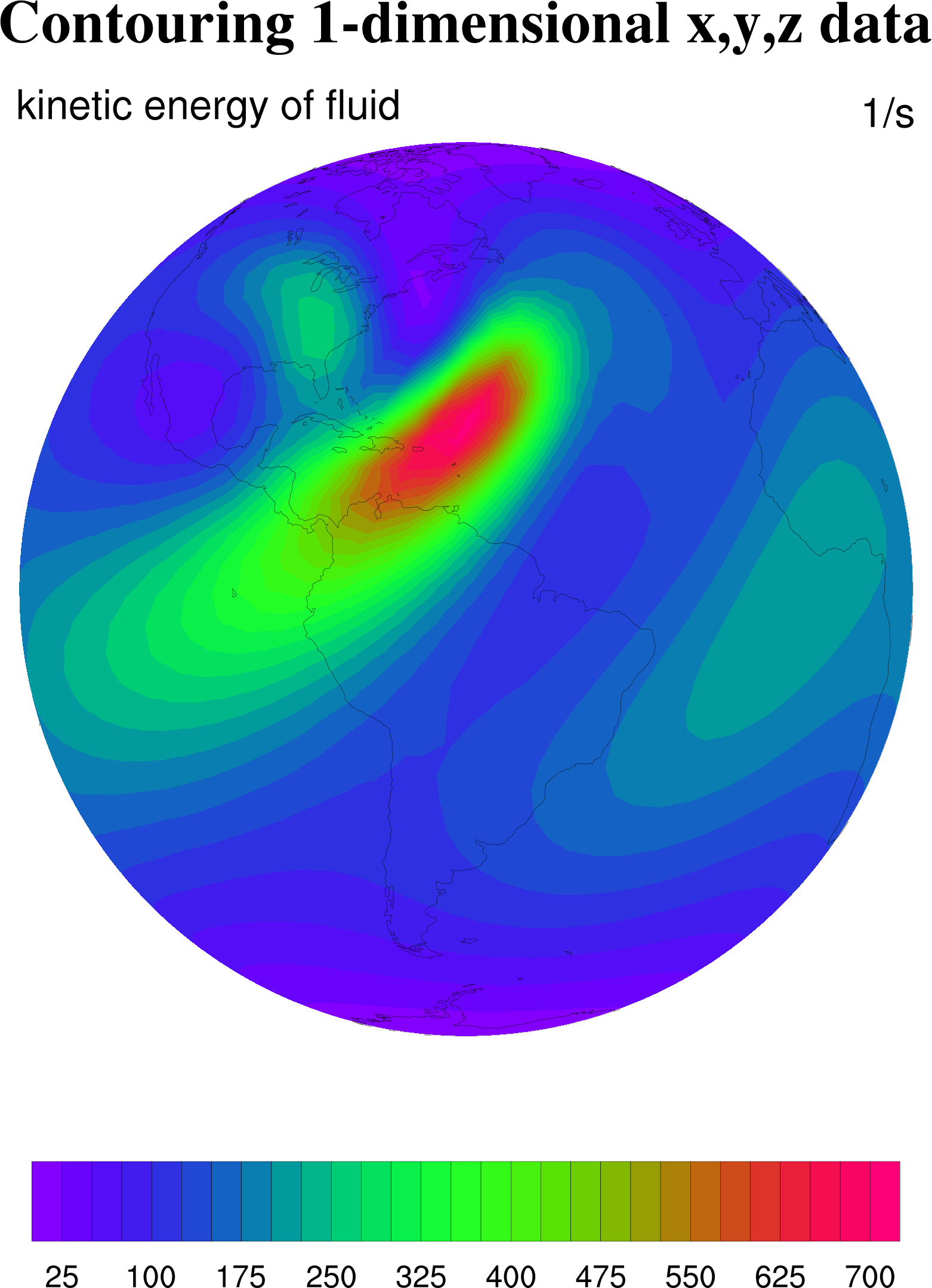
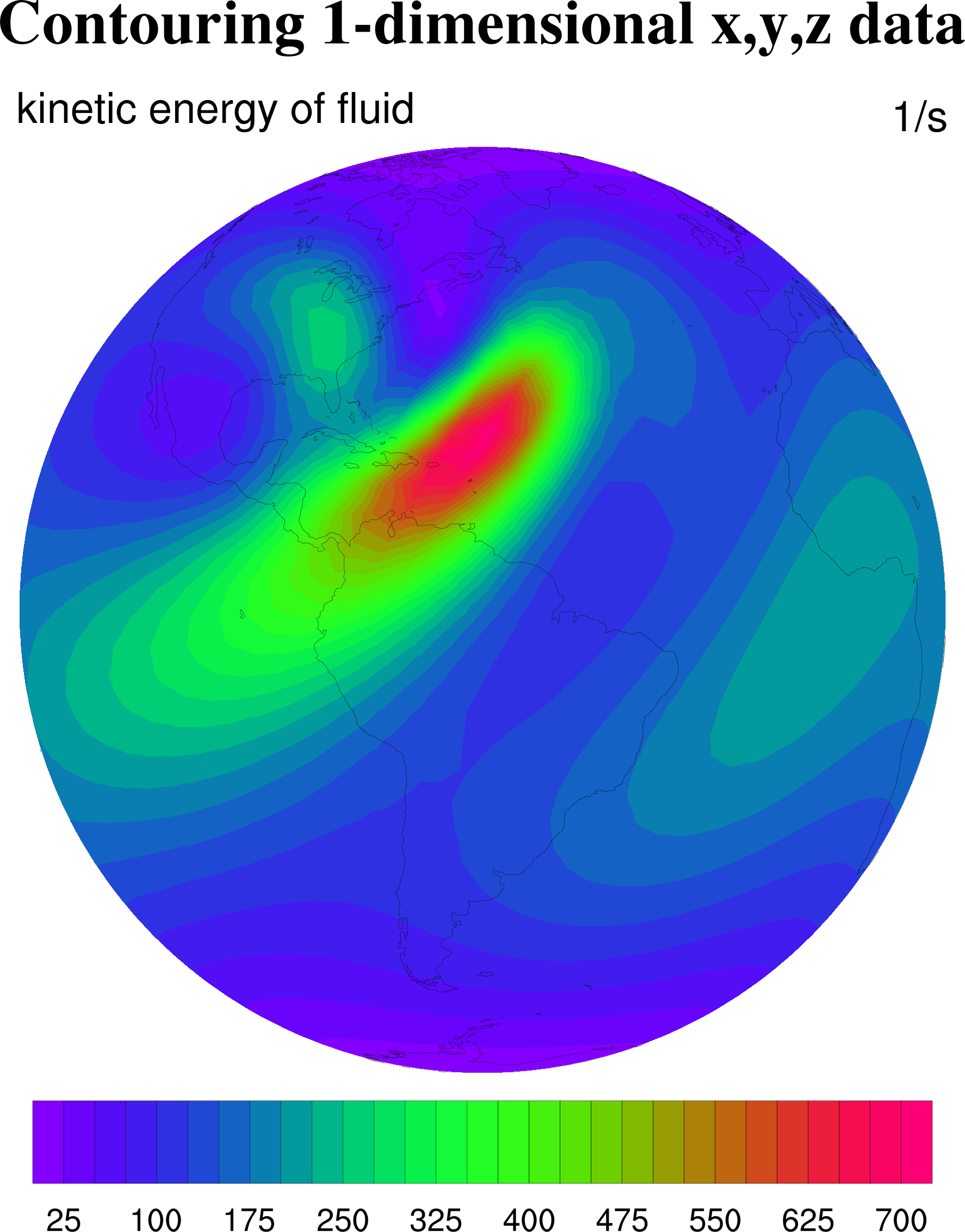
contouring
| 
| 
| 
|
| contour1a.ncl | contour1b.ncl | contour1c.ncl | contour1d.ncl |
| 
| ||
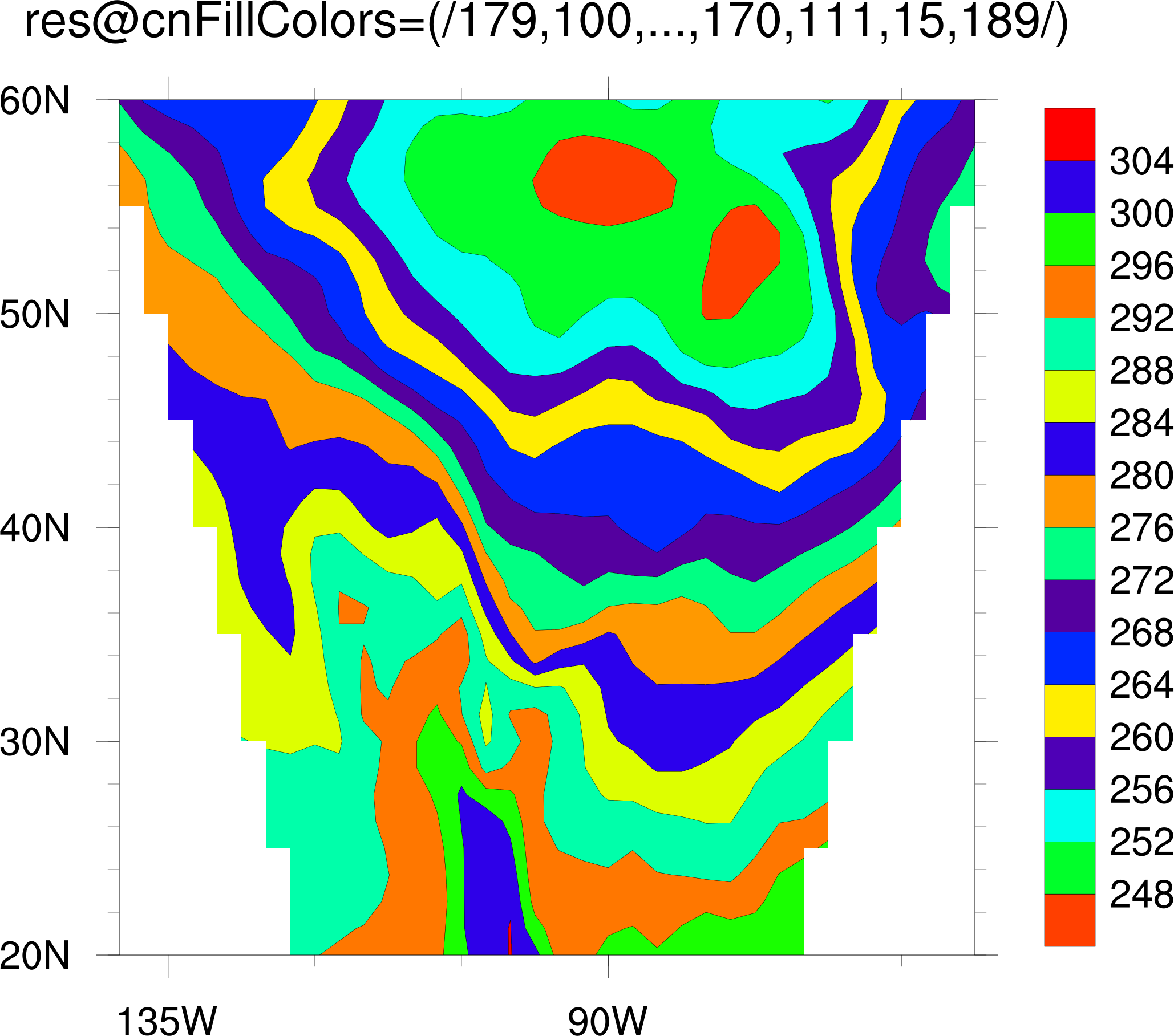
| contour1e.ncl | contour1d_levels.ncl |
contouring curvilinear data (2D lat/lon arrays)
| 
| 
| 
|
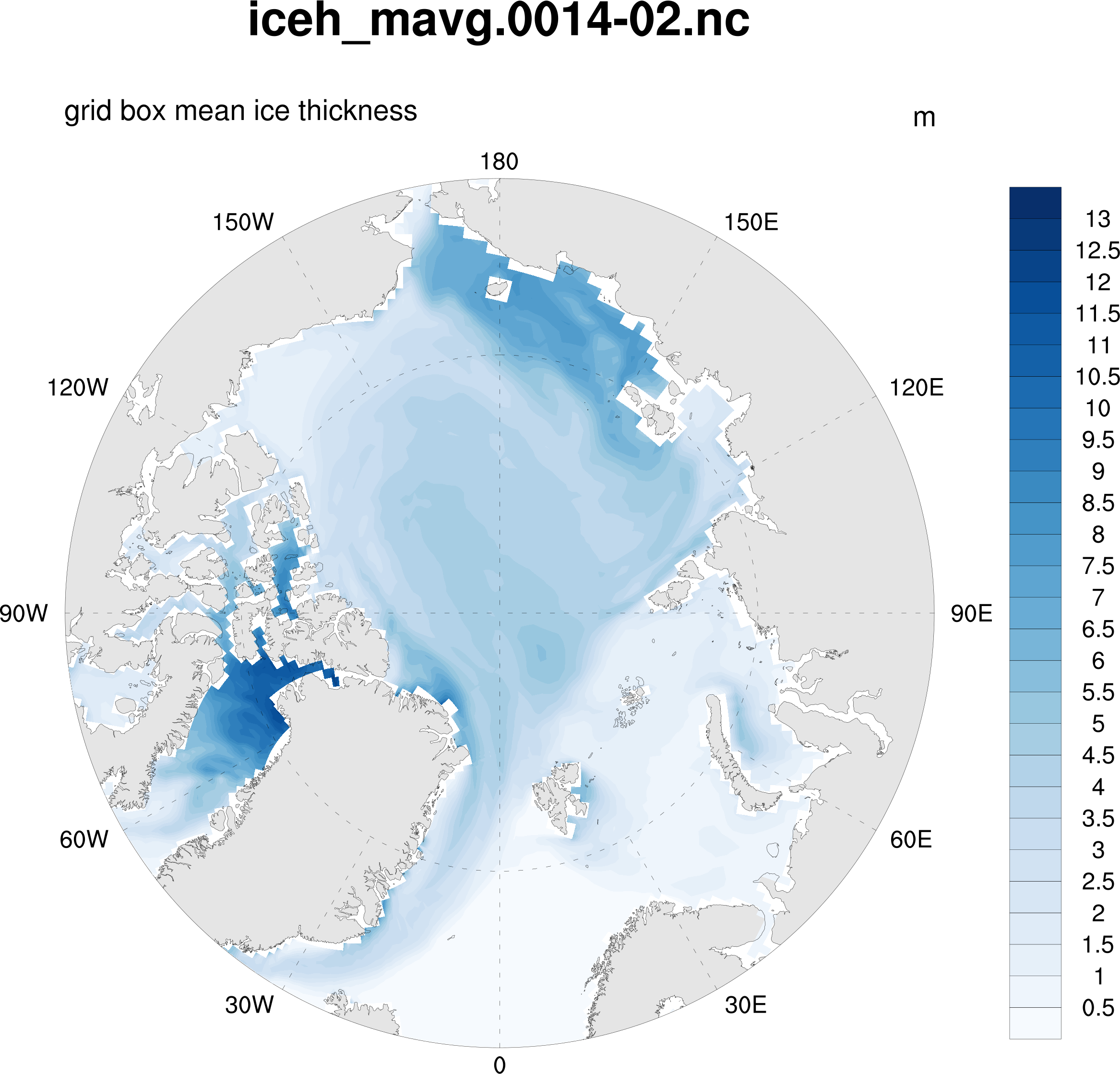
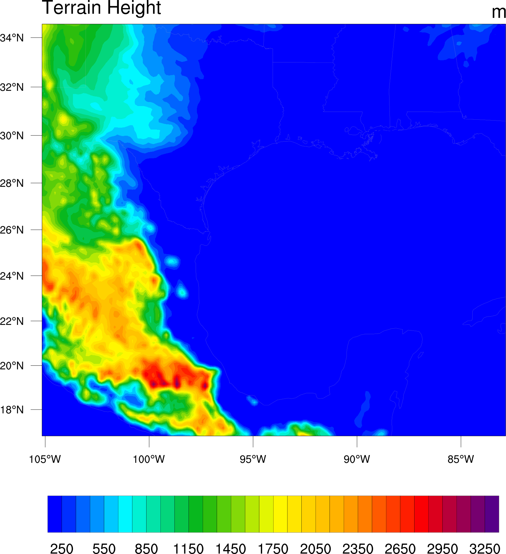
| ice.ncl | wrfgeo_gsn.ncl | contour4d.ncl | contour6f.ncl |
| |||
| contour7i.ncl |
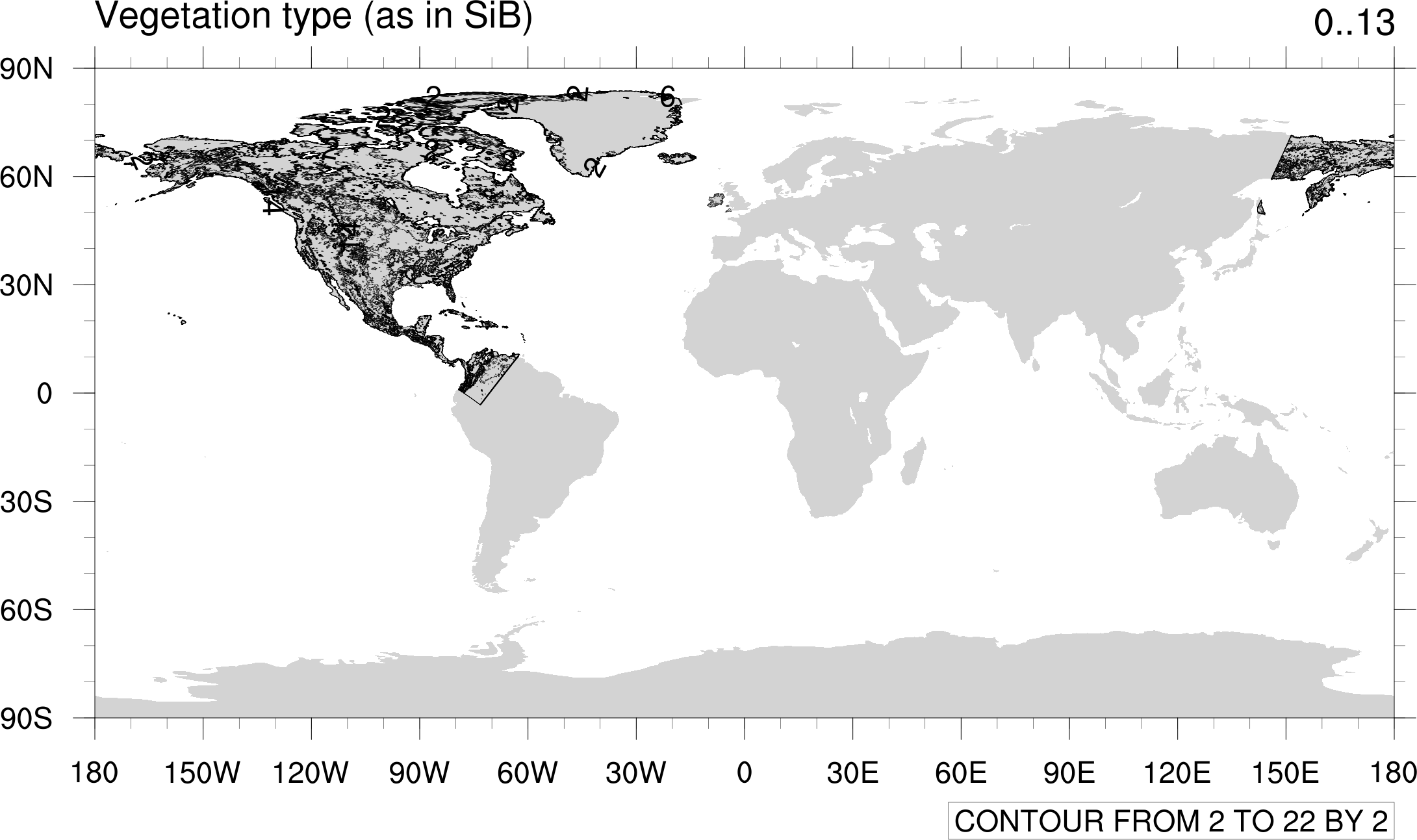
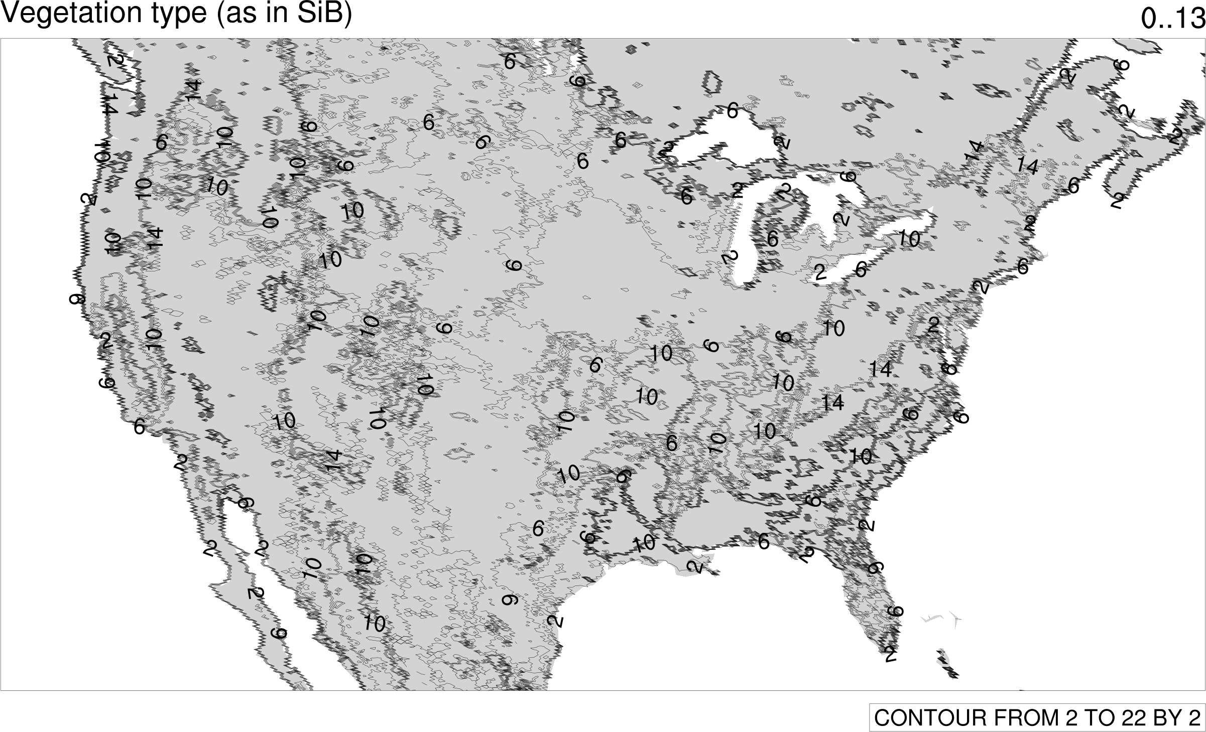
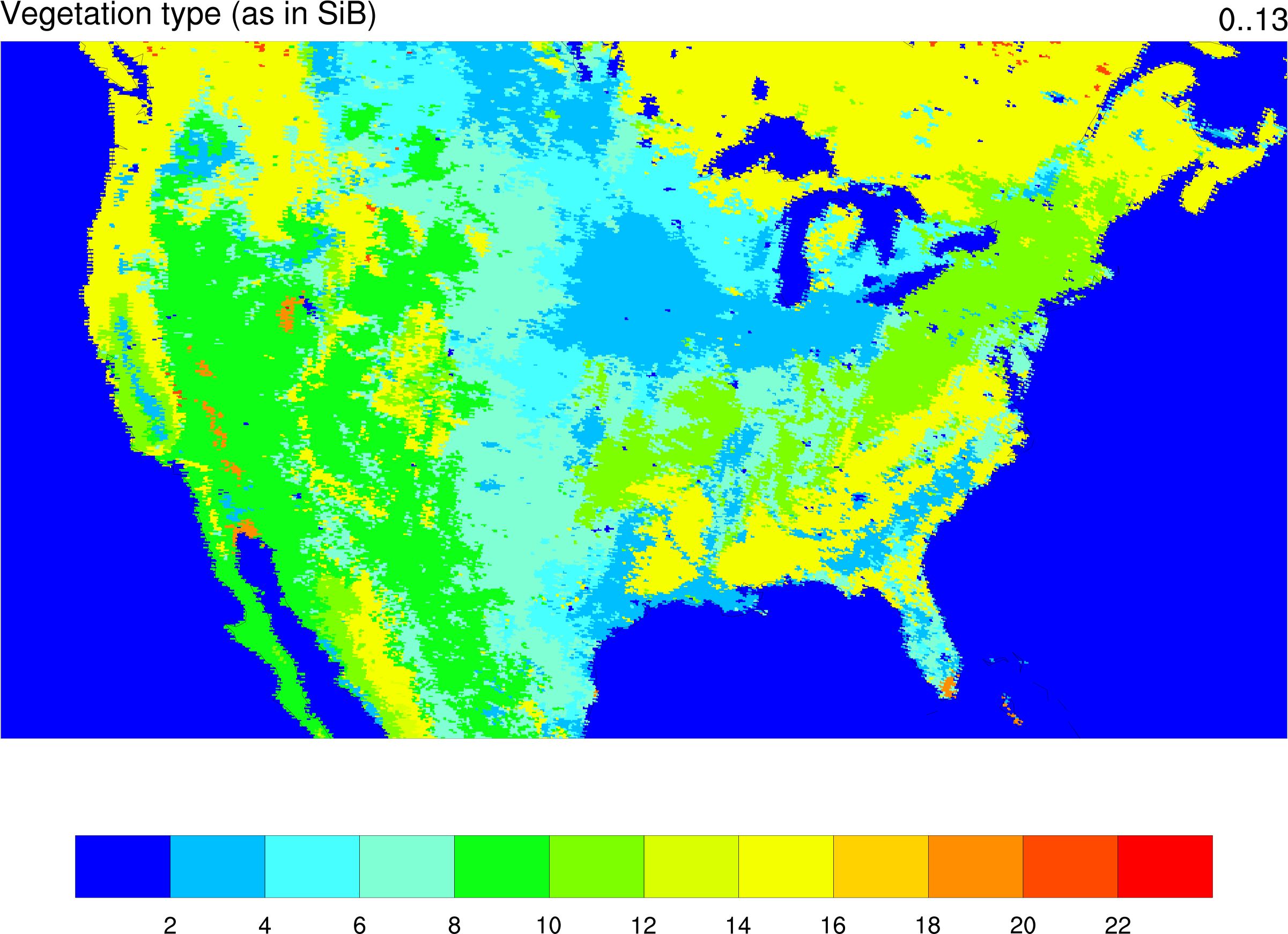
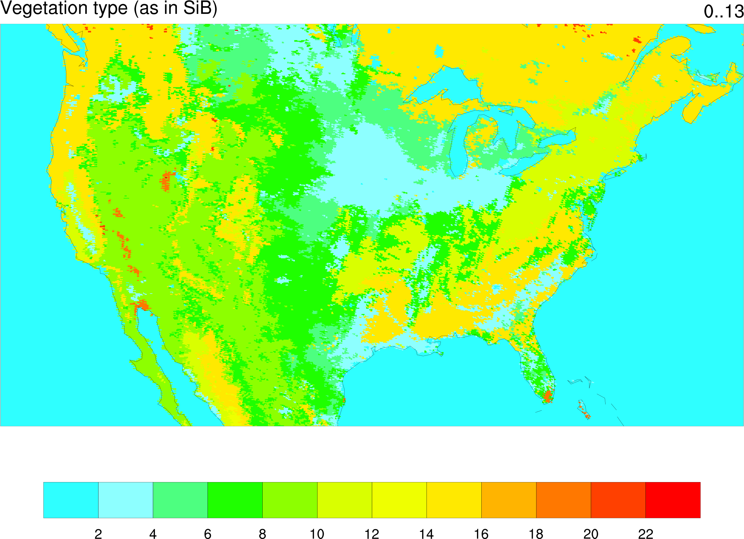
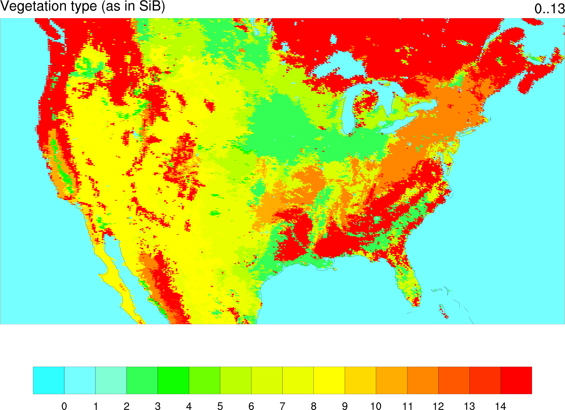
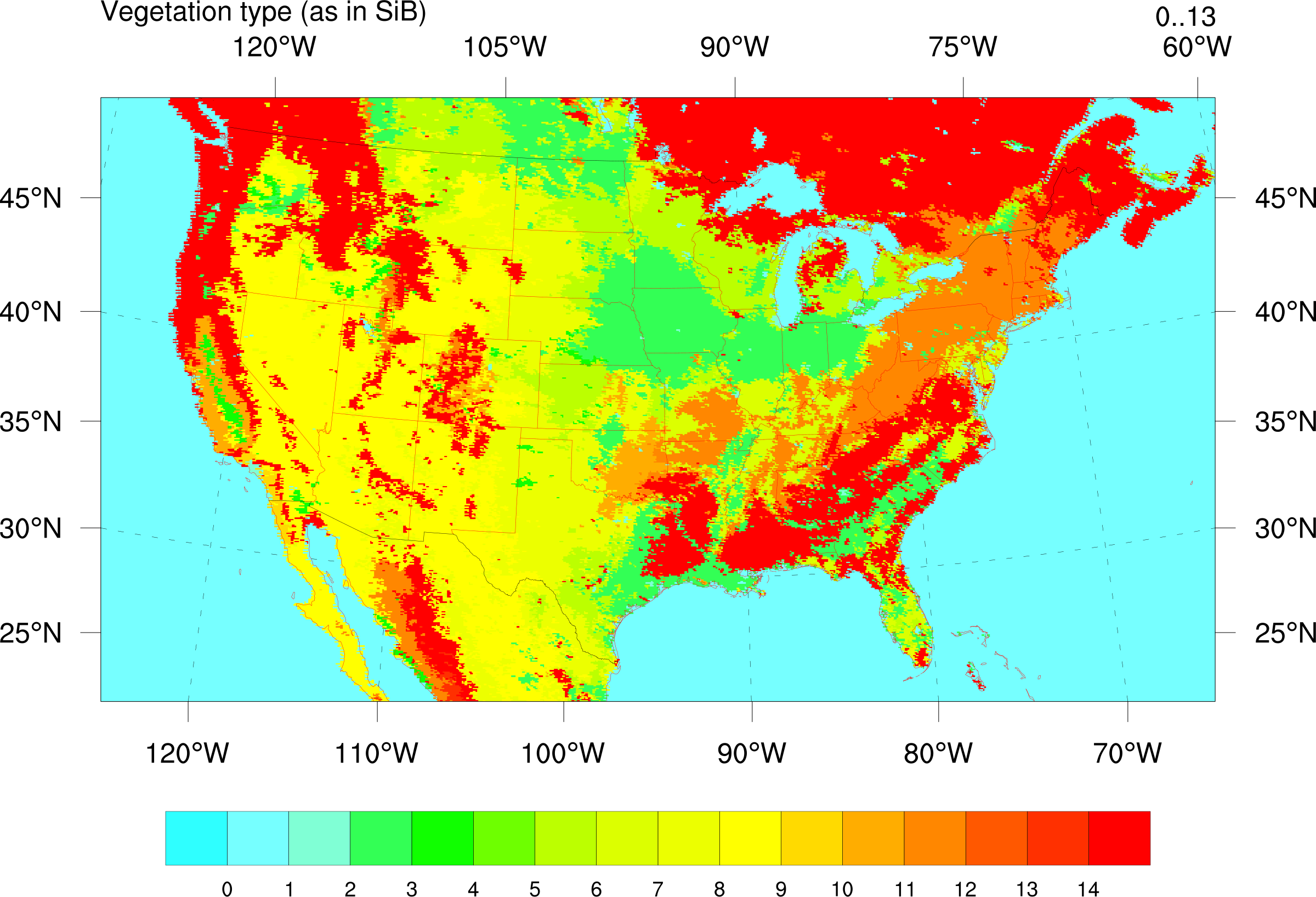
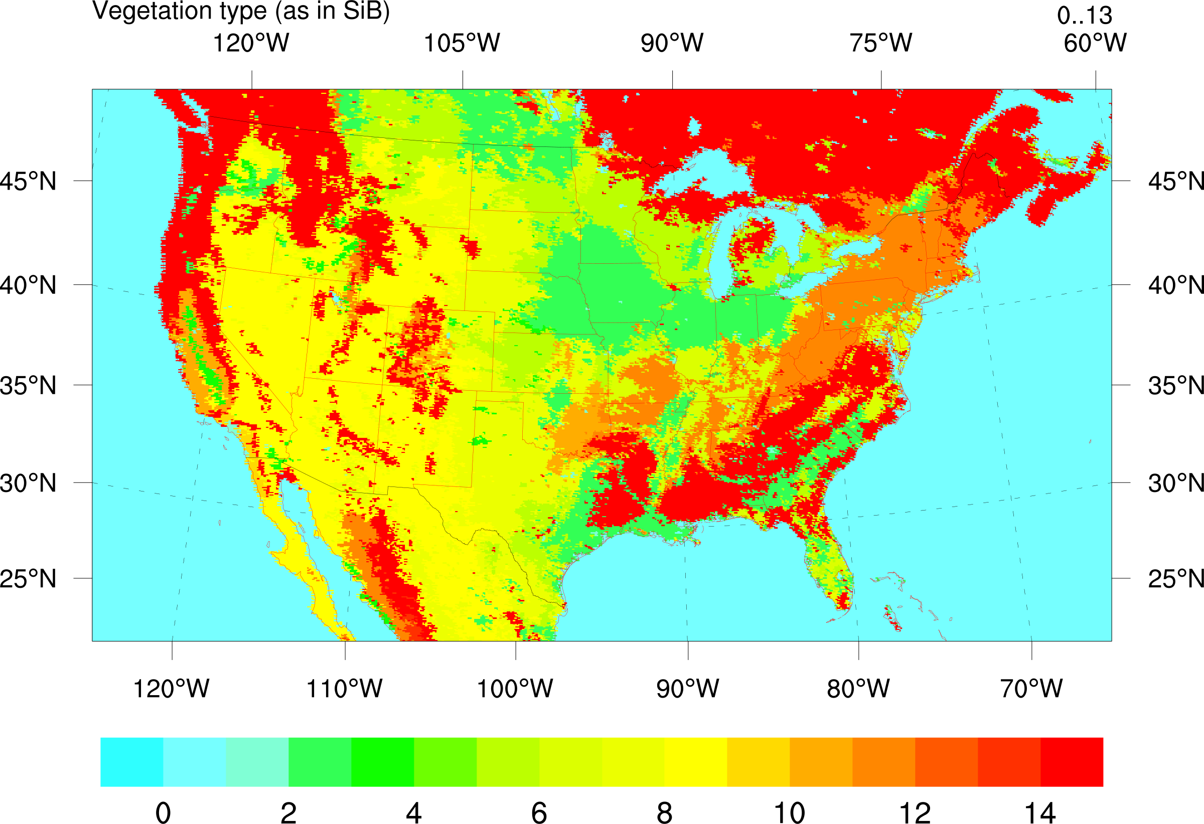
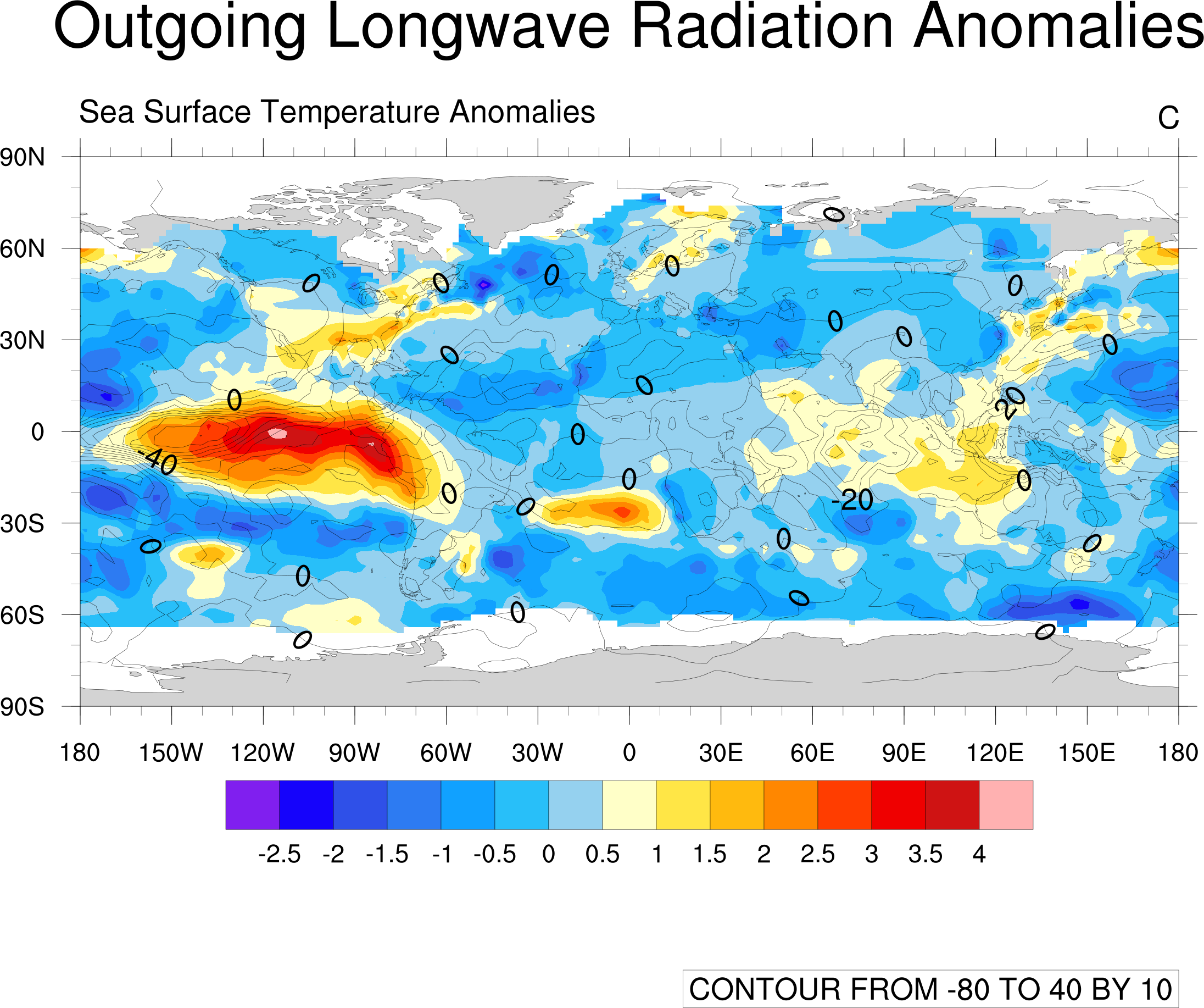
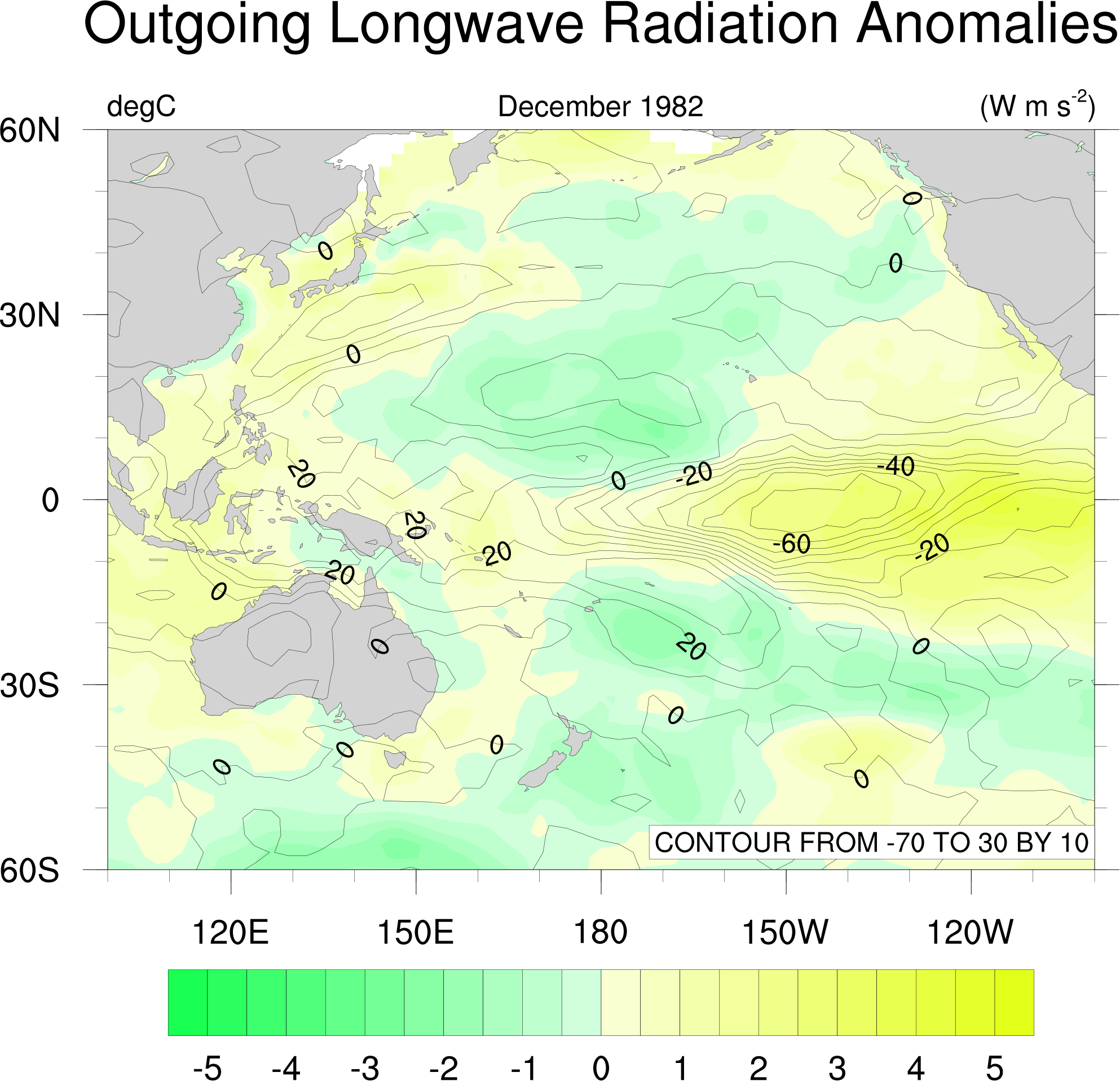
contouring over cylindrical equidistant maps
| 
| 
| 
|
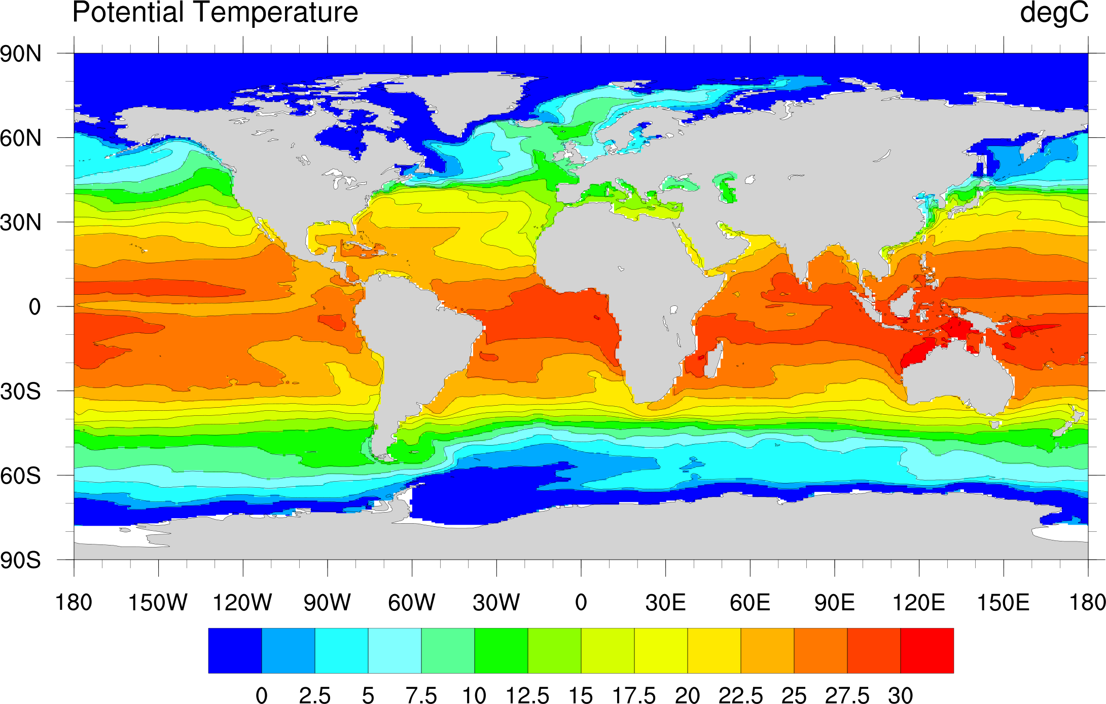
| contour2a.ncl | contour2b.ncl | contour2c.ncl | contour2d.ncl |
| 
| 
| 
|
| contour2e.ncl | contour4a.ncl | contour4b.ncl | contour4c.ncl |
|
| |||
| contour4d.ncl |
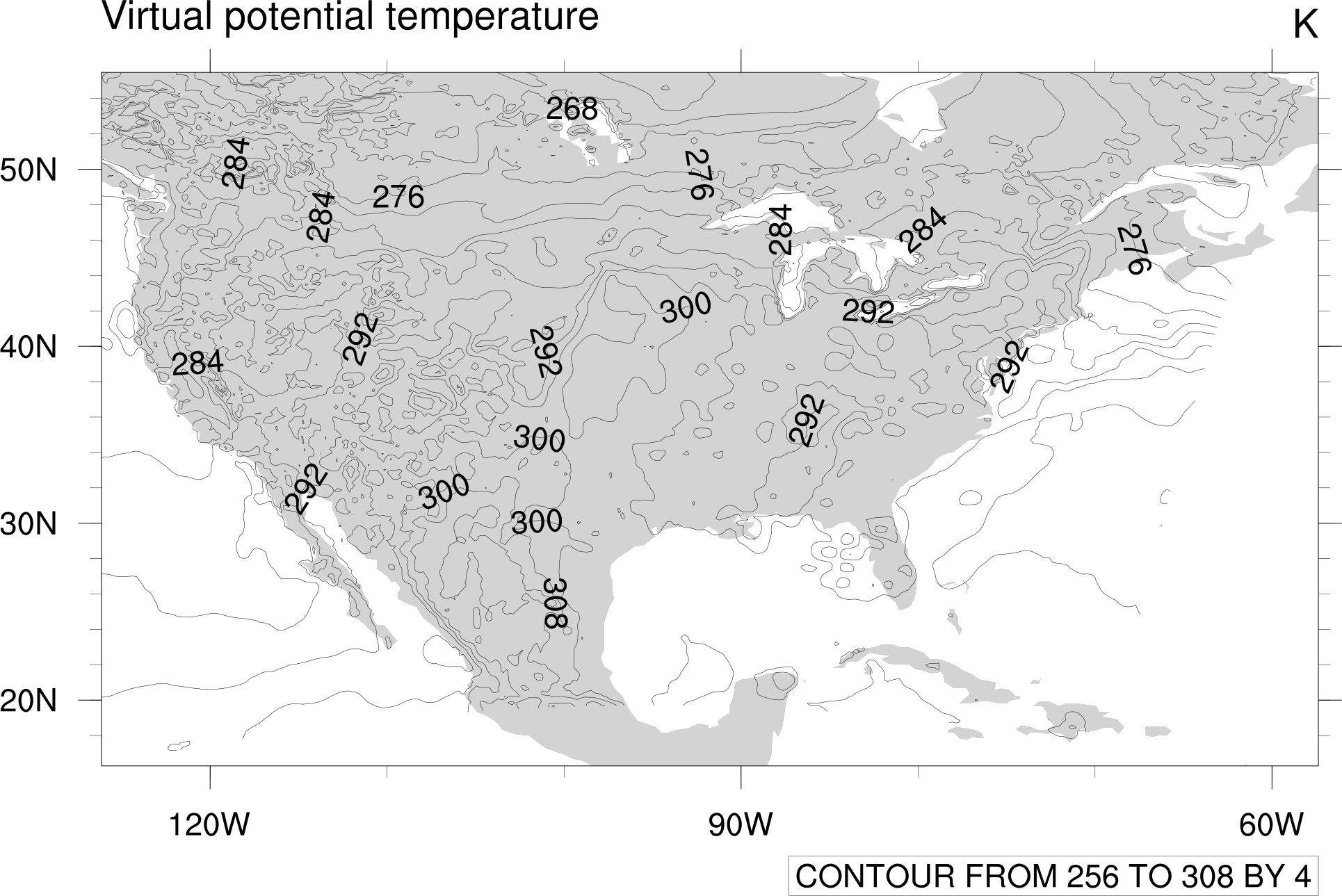
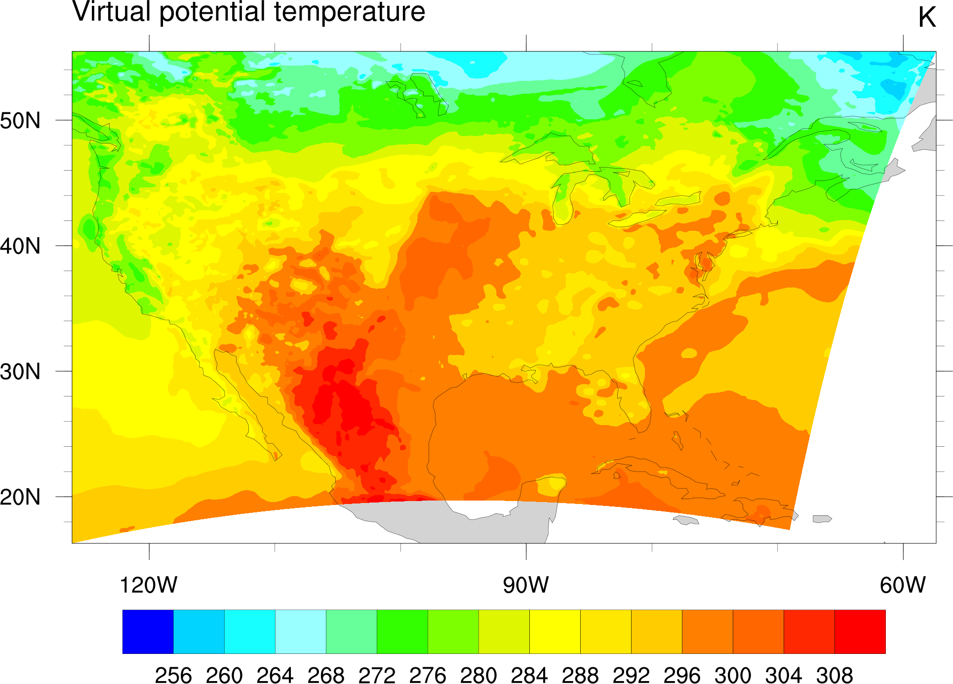
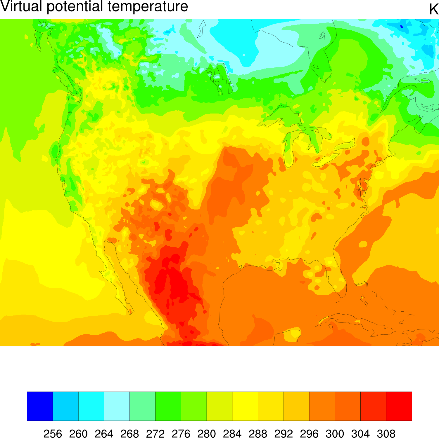
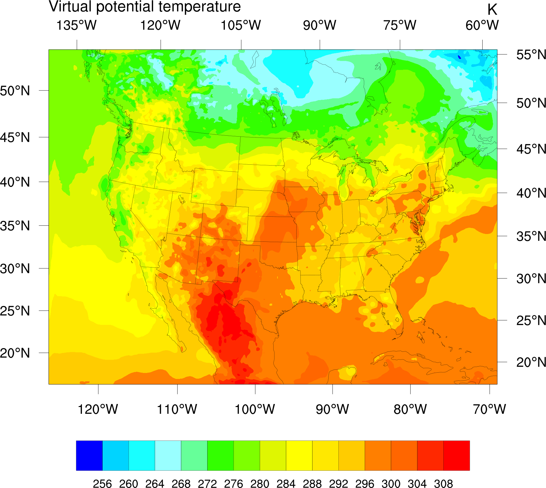
contouring over lambert conformal maps

contouring rectilinear data (1D lat/lon coordinate arrays)
|
| 
| 
|
| contour2e.ncl | contour3d.ncl | contour9a.ncl |
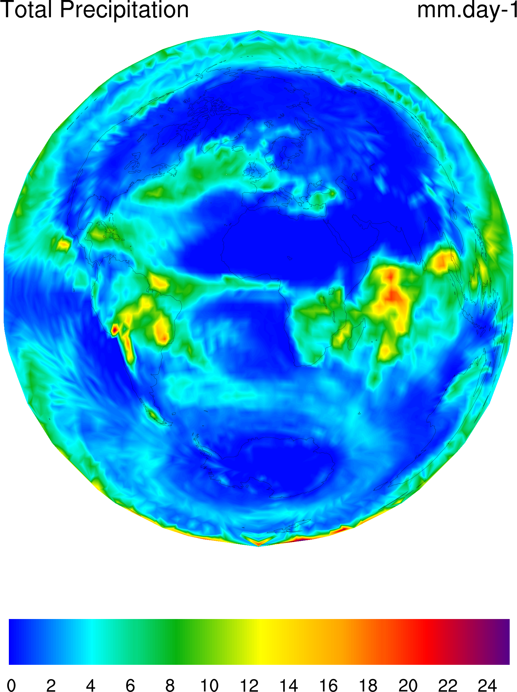
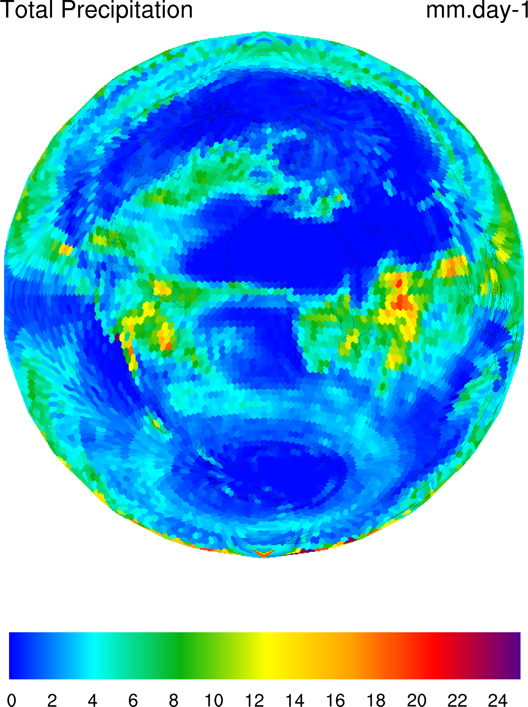
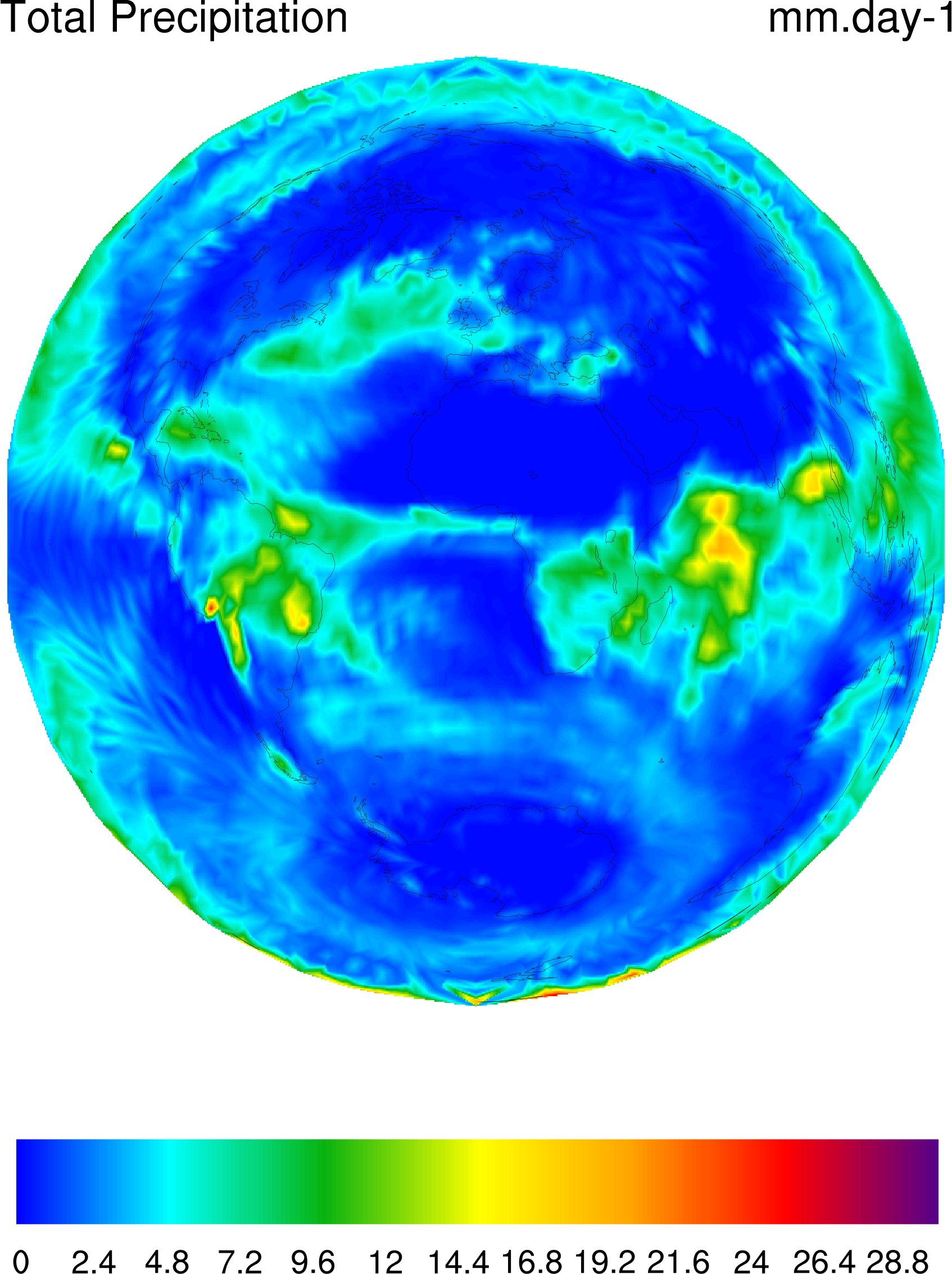
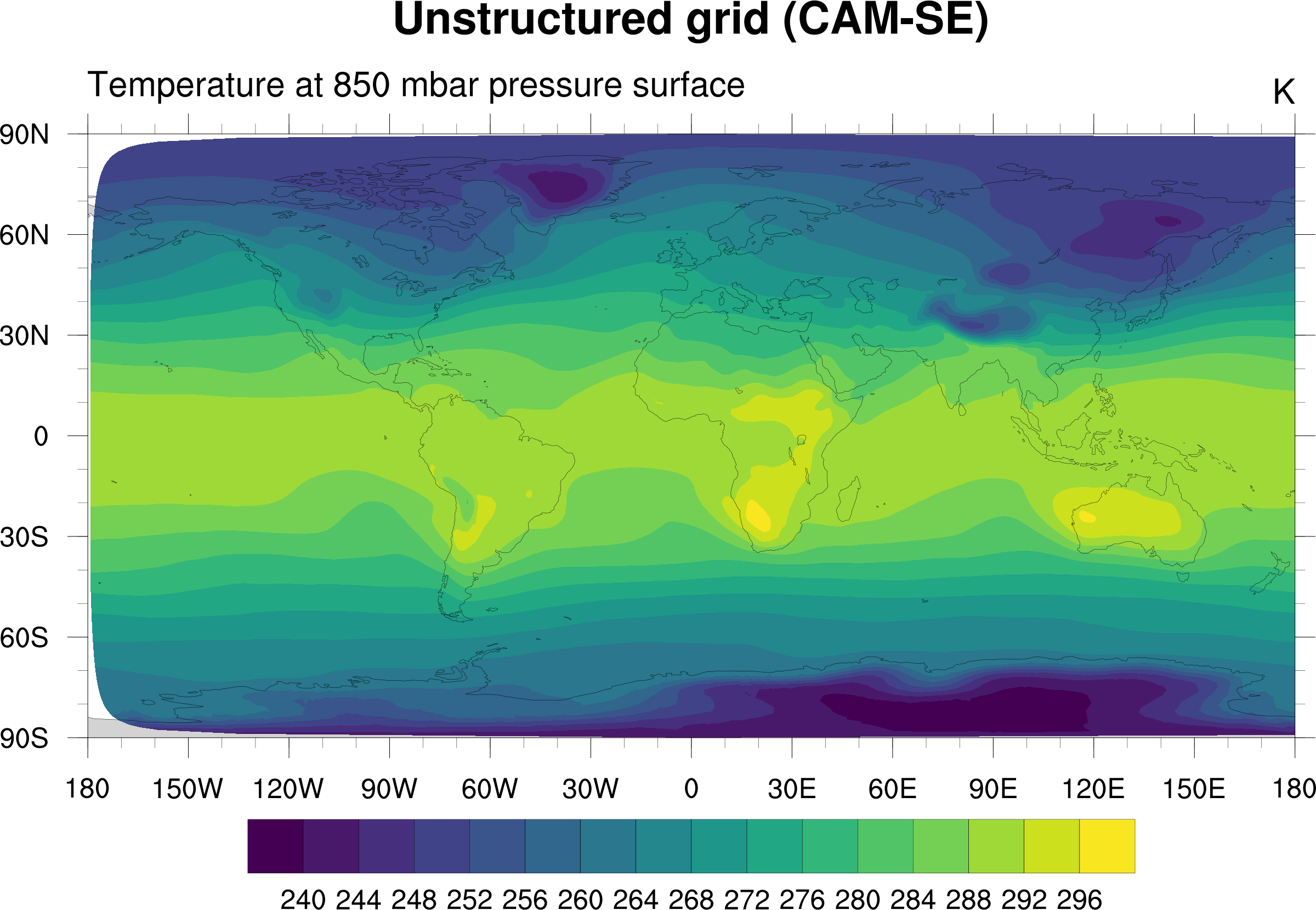
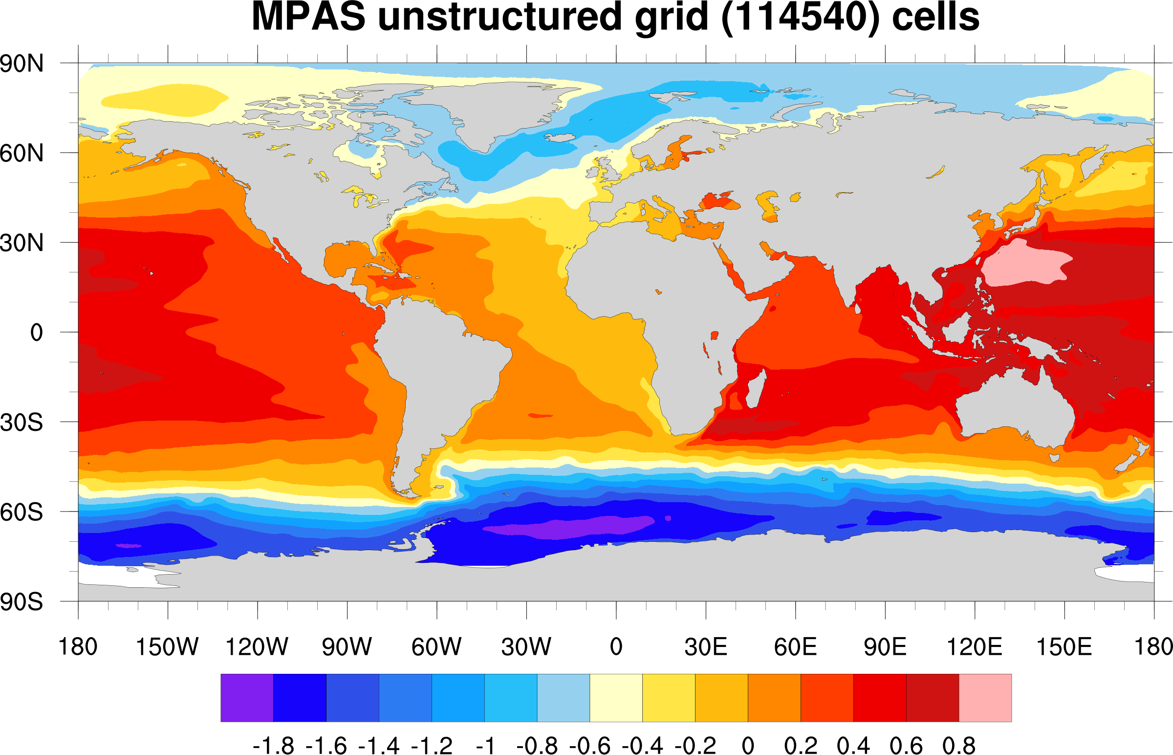
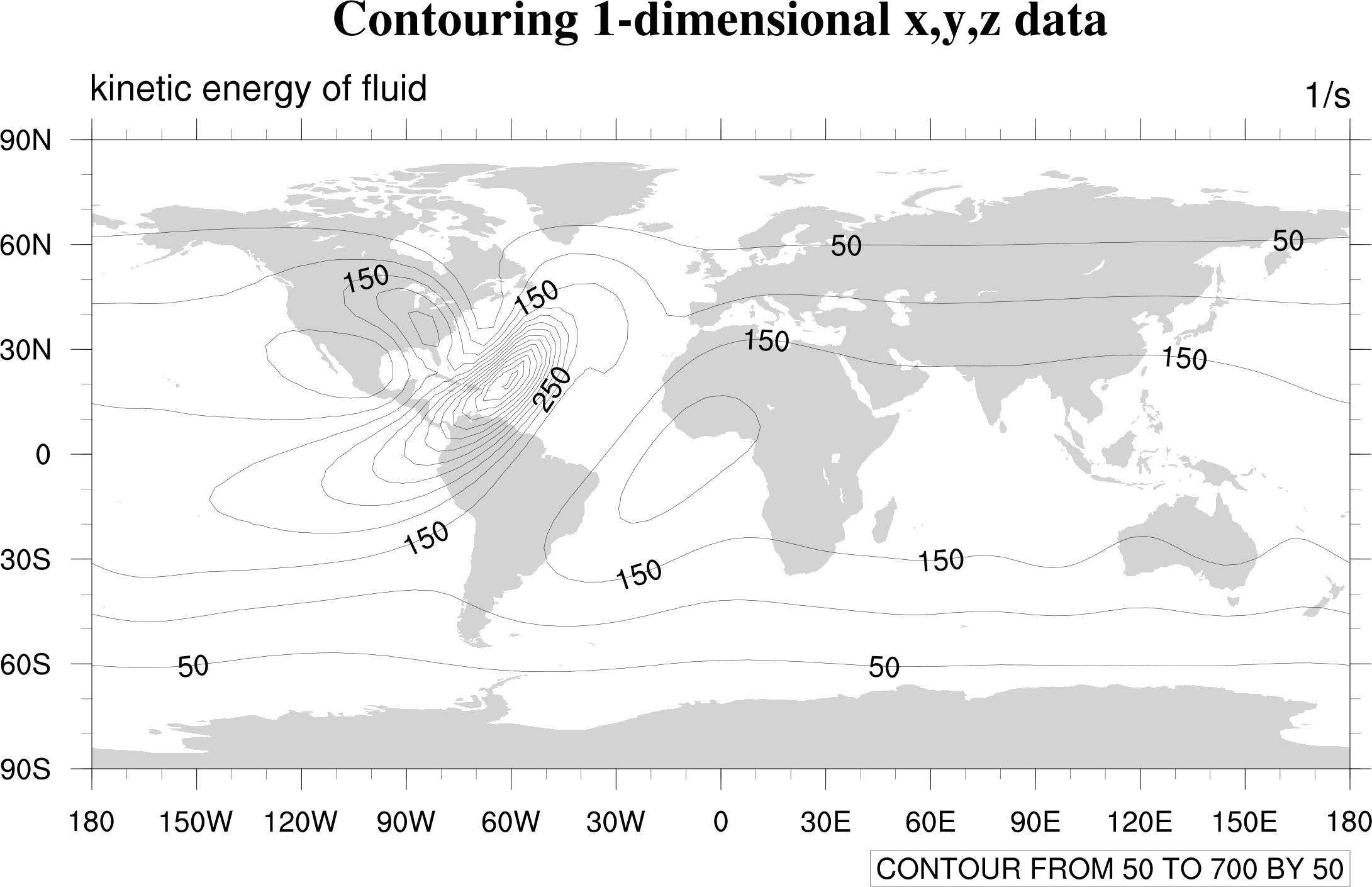
contouring unstructured data
| 
| 
| 
|
| arpege_smooth.ncl | arpege_raster.ncl | arpege_raster_smooth.ncl | arpege_raster_smooth_640.ncl |
| 
| 
| 
|
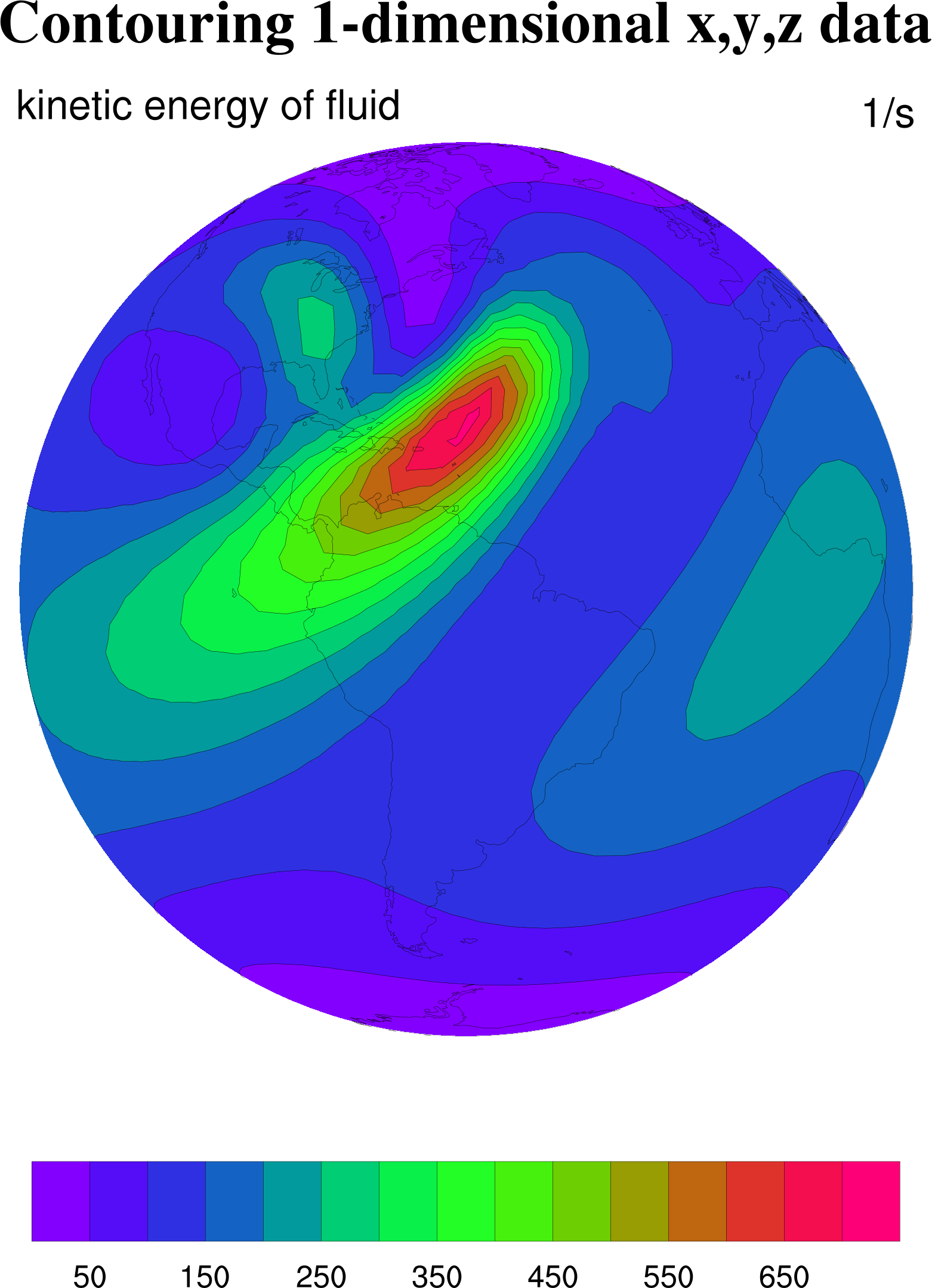
| camse.ncl | camse_640.ncl | mpas.ncl | contour5a.ncl |

| 
| 
| 
|
| contour5b.ncl | contour5c.ncl | contour5d.ncl | contour5e.ncl |
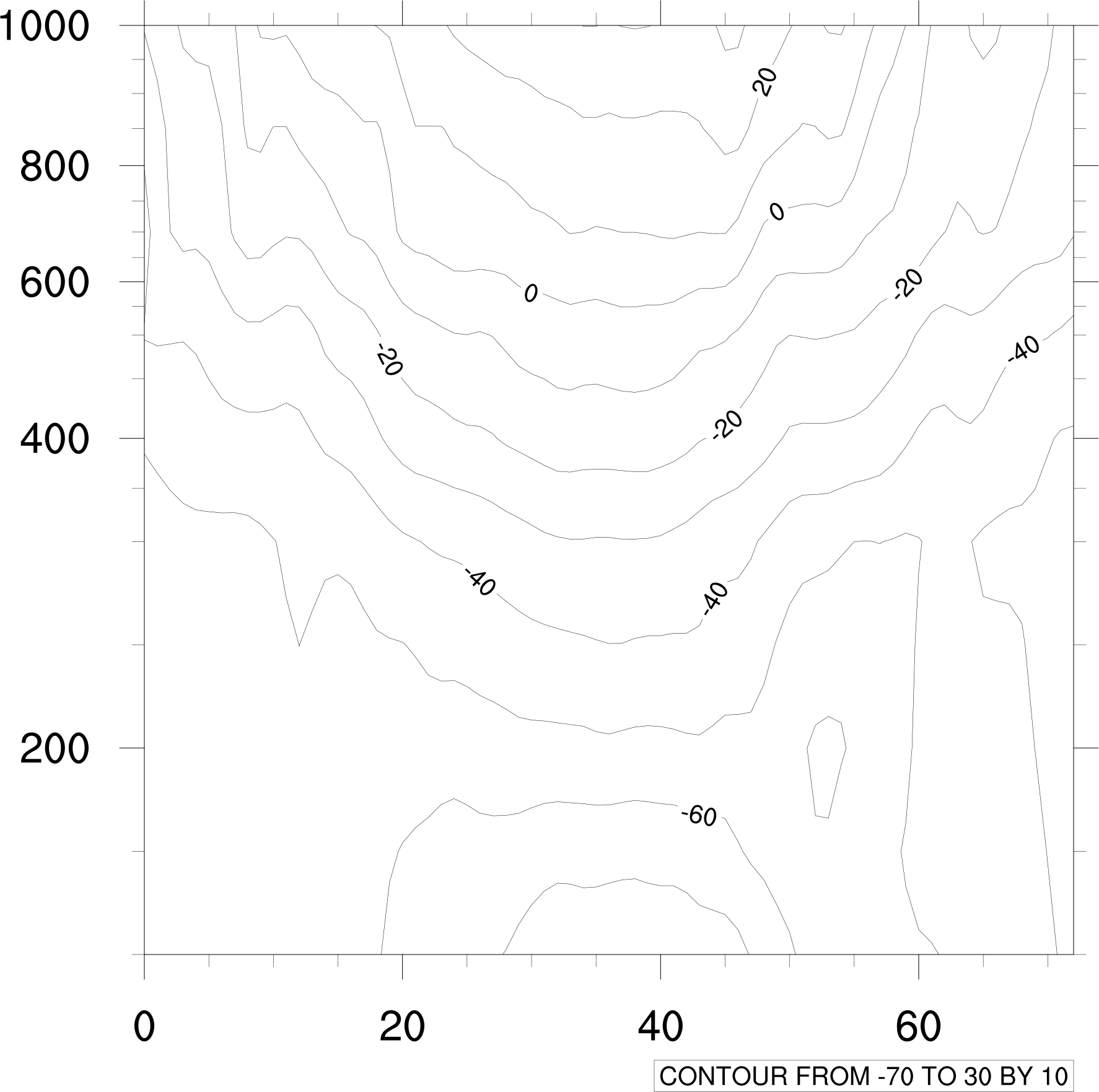
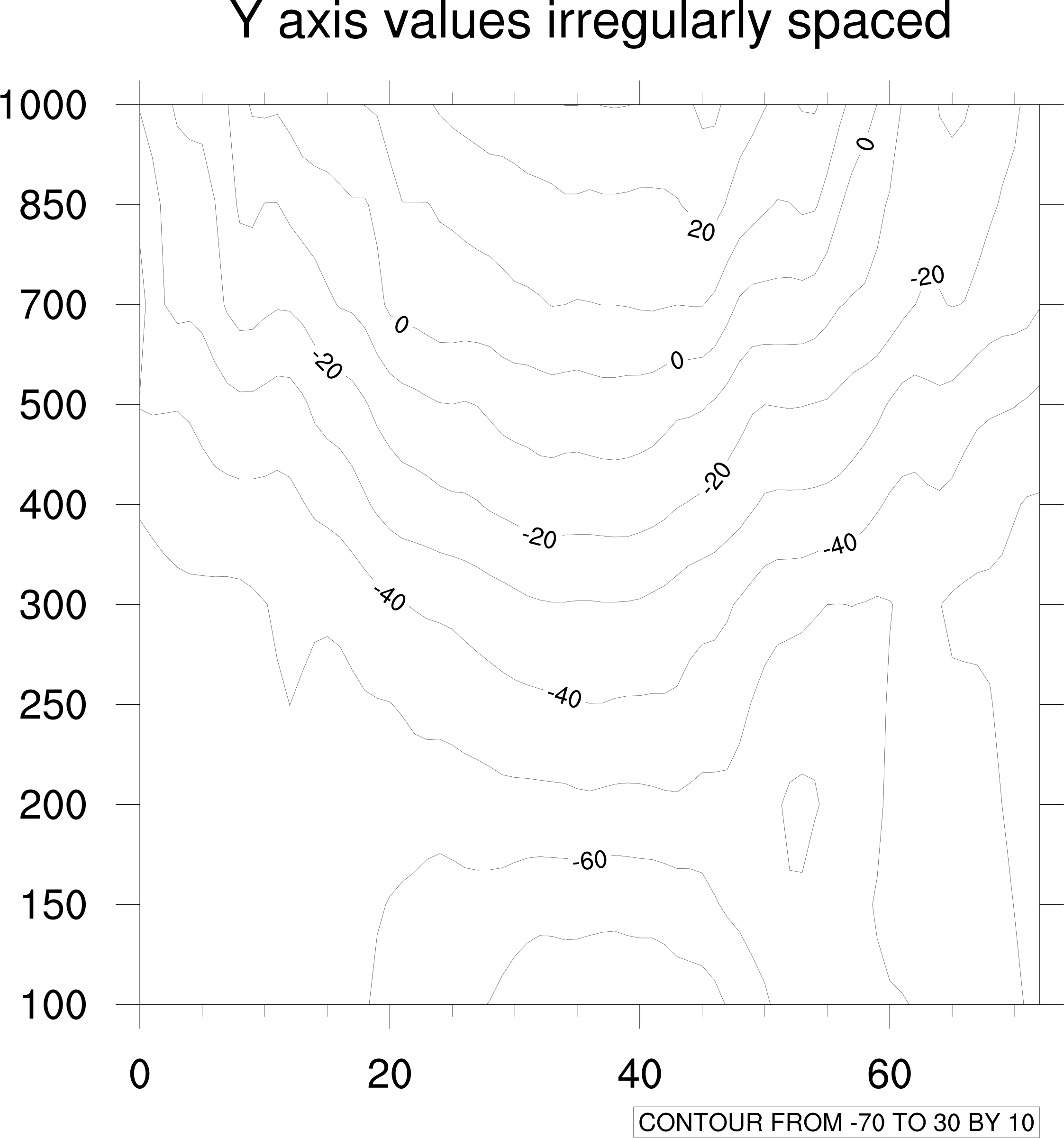
contouring with irregular coordinate arrays
| 
| 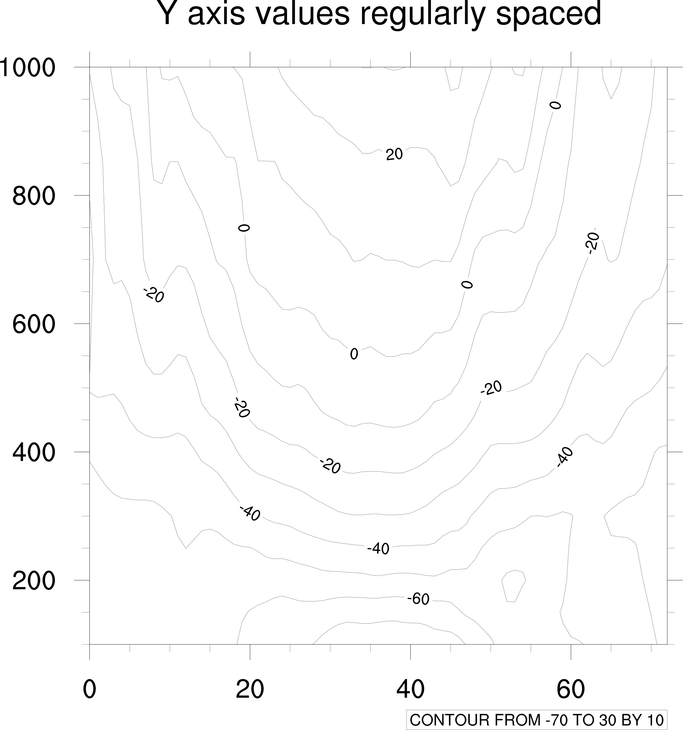
| 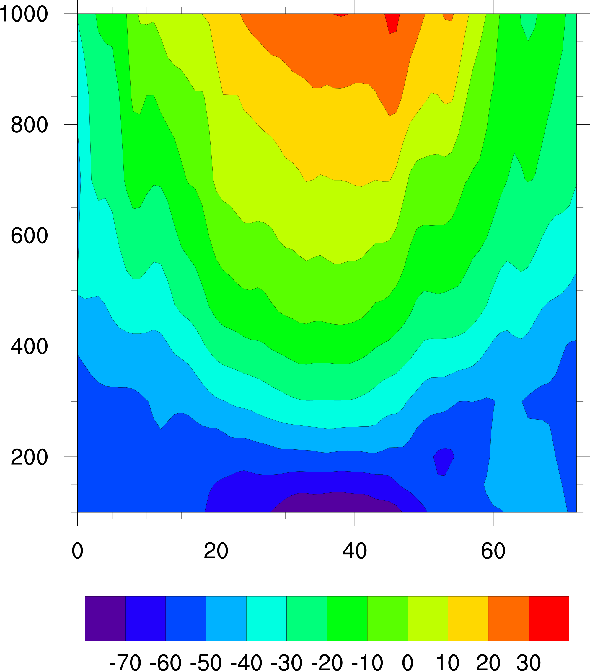
|
| irregular1a.ncl | irregular1b.ncl | irregular1c.ncl | irregular1d.ncl |
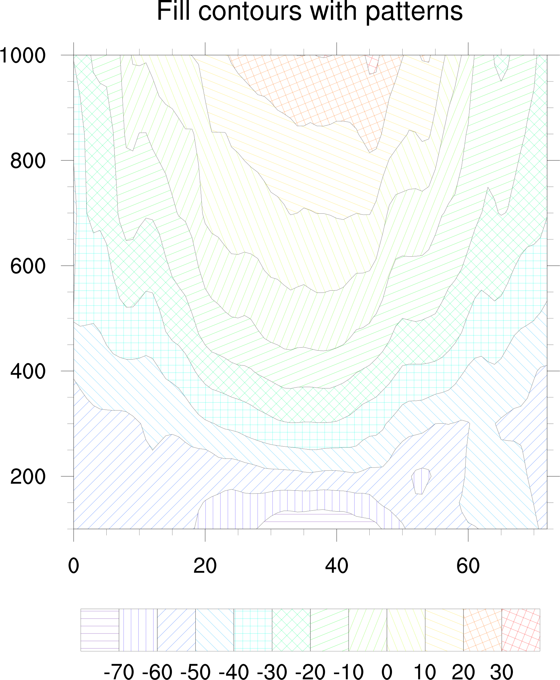
| 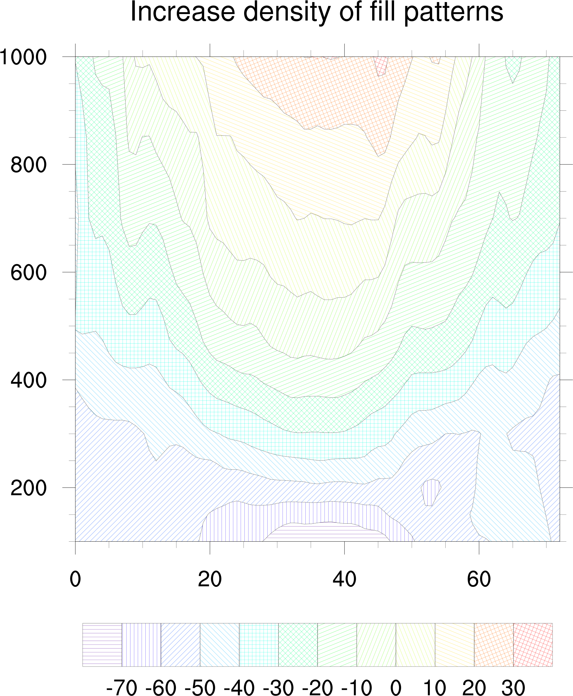
| 
| 
|
| irregular1e.ncl | irregular1f.ncl | irregular1g.ncl | irregular1h.ncl |
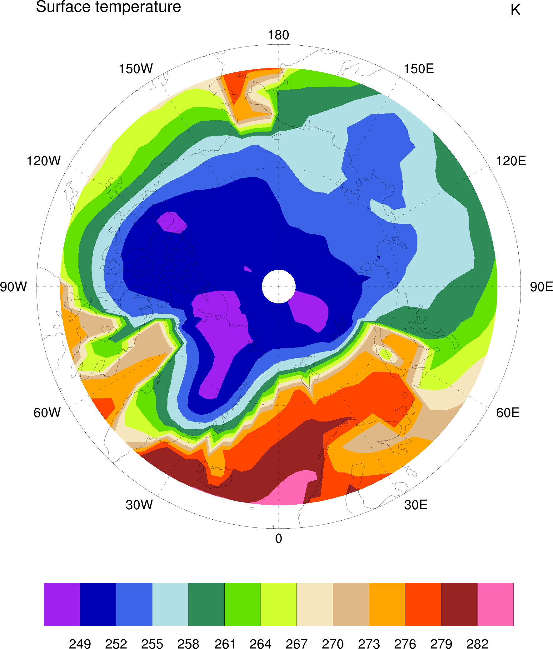
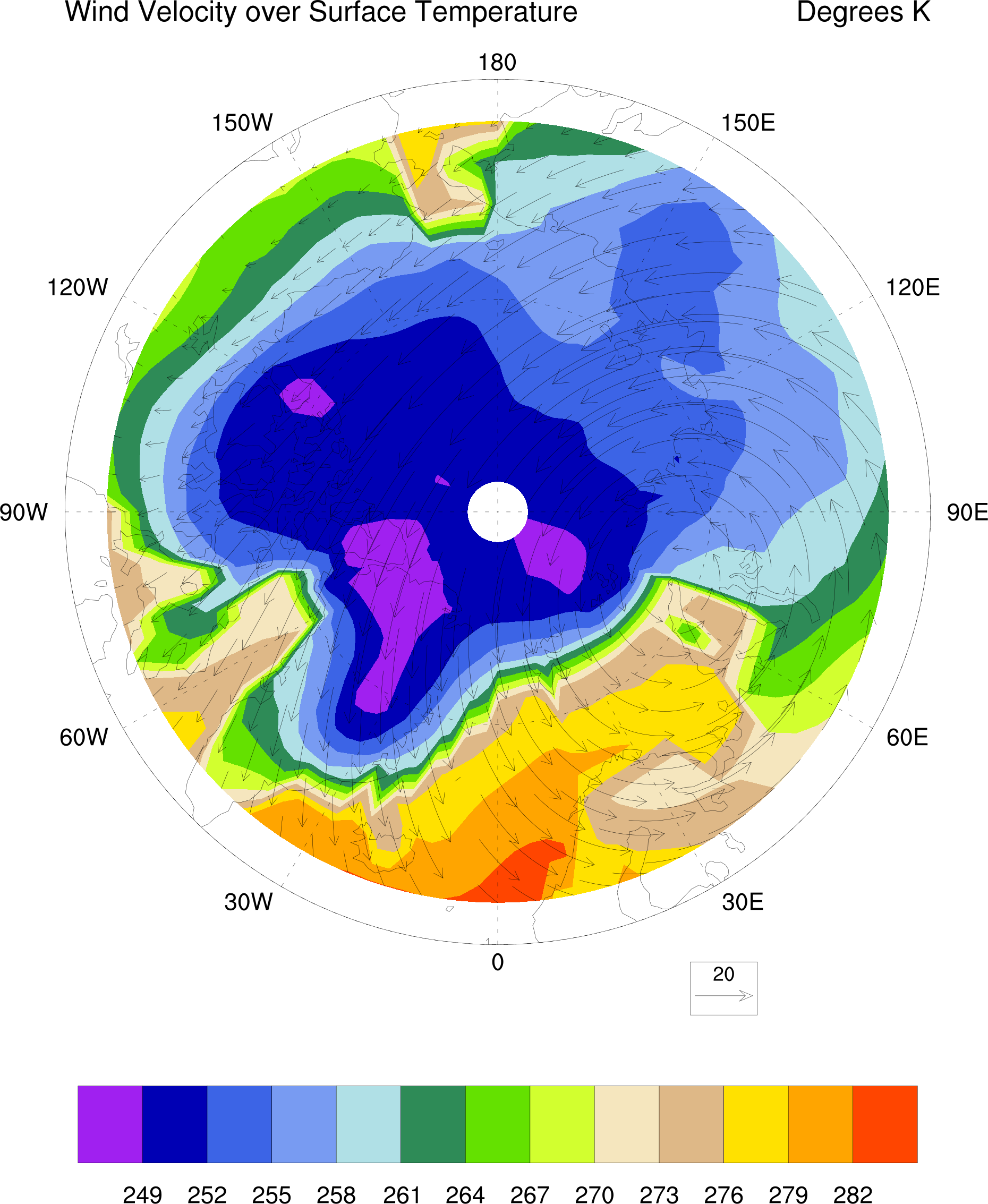
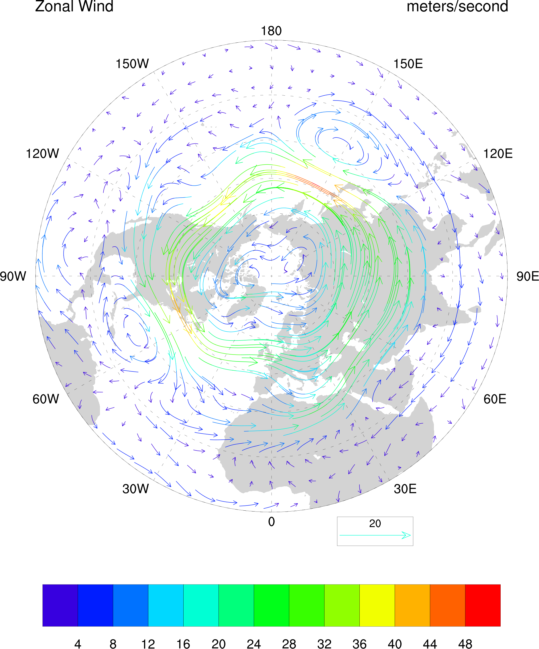
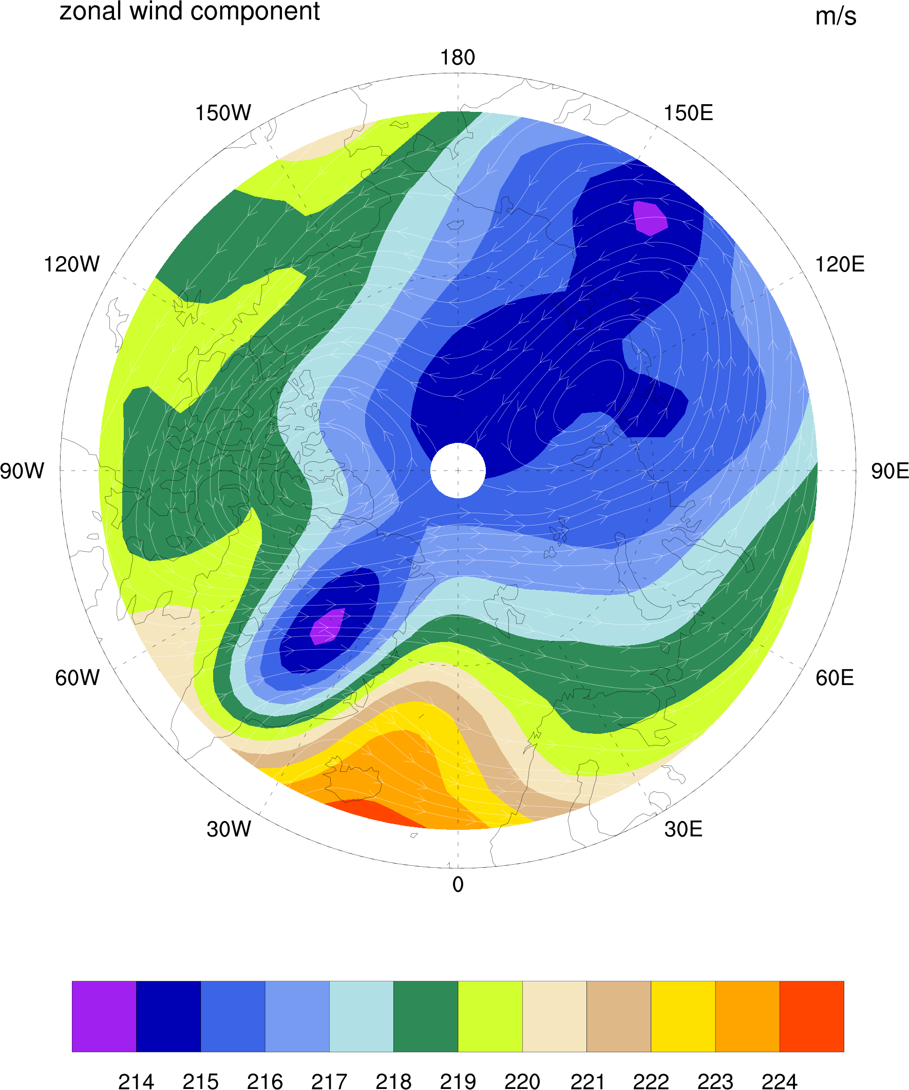
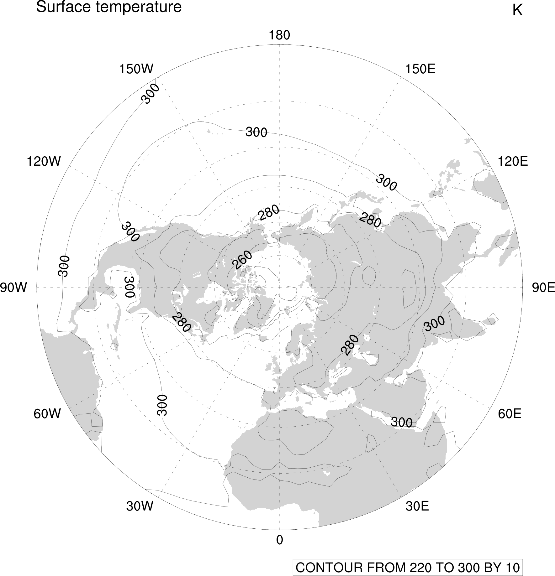
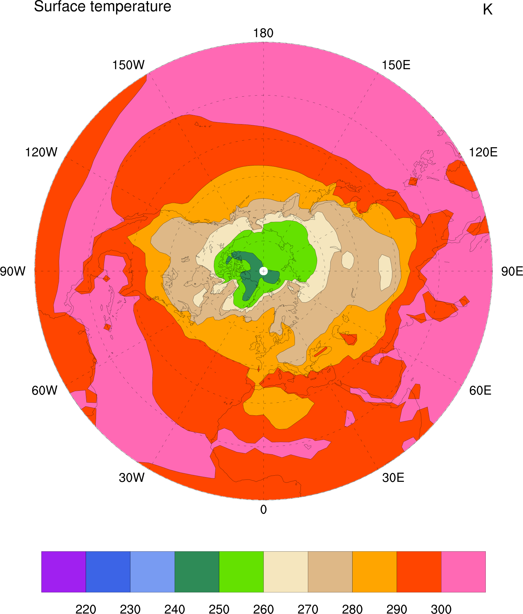
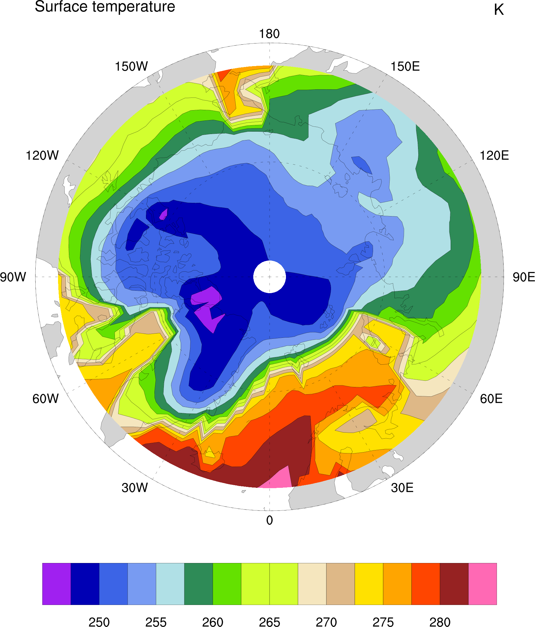
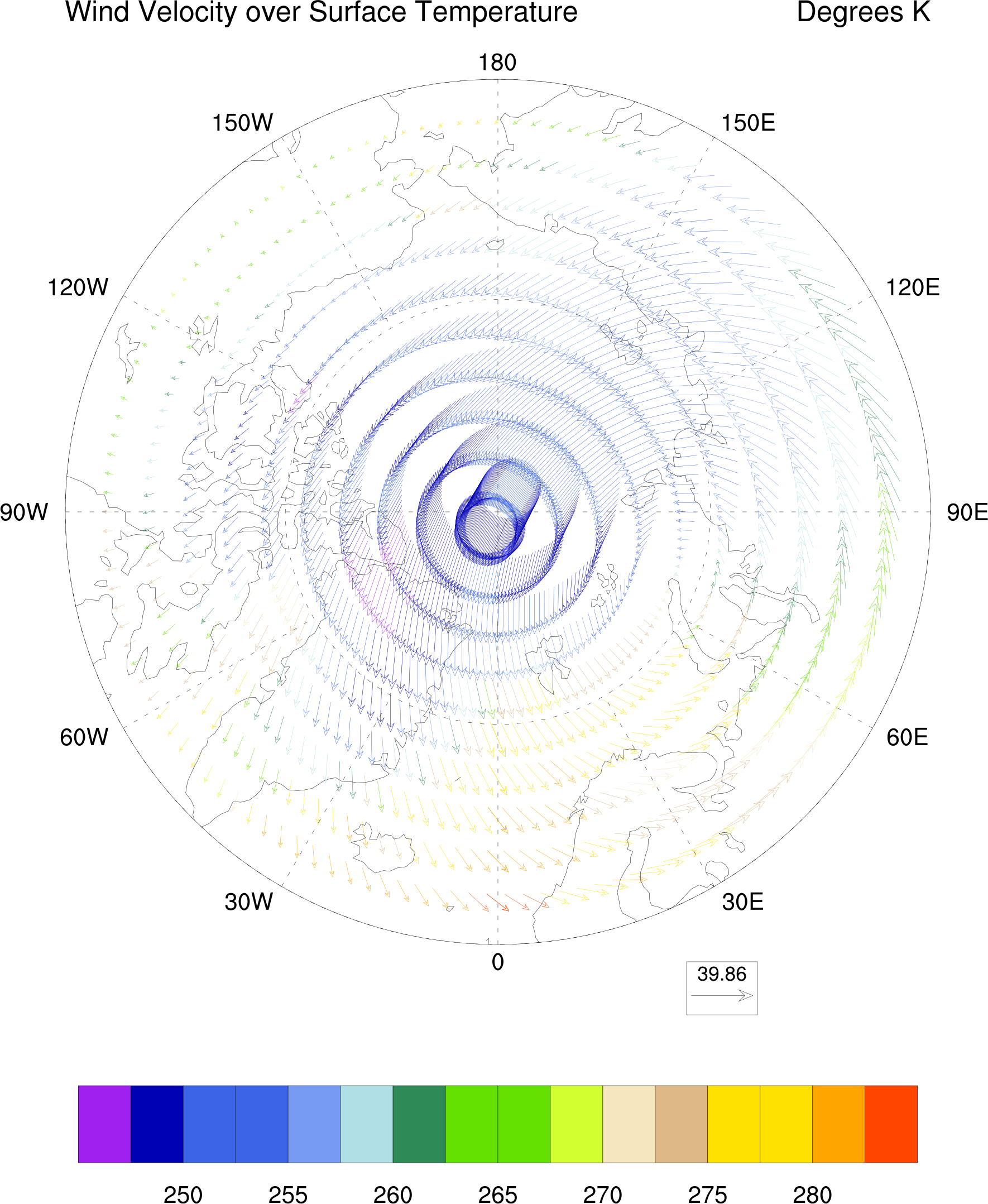
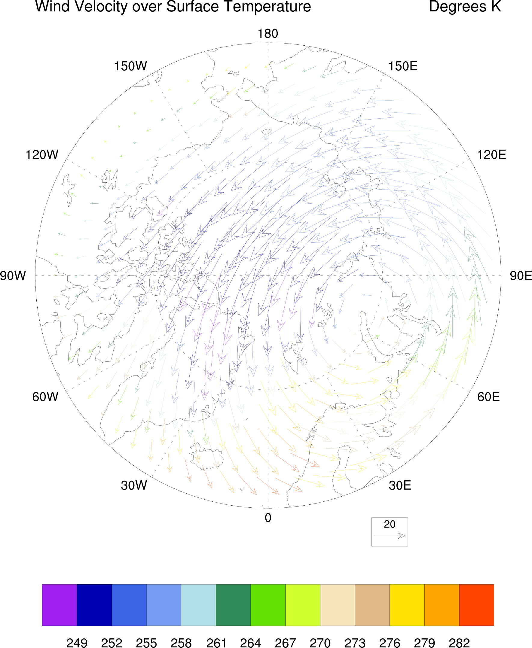
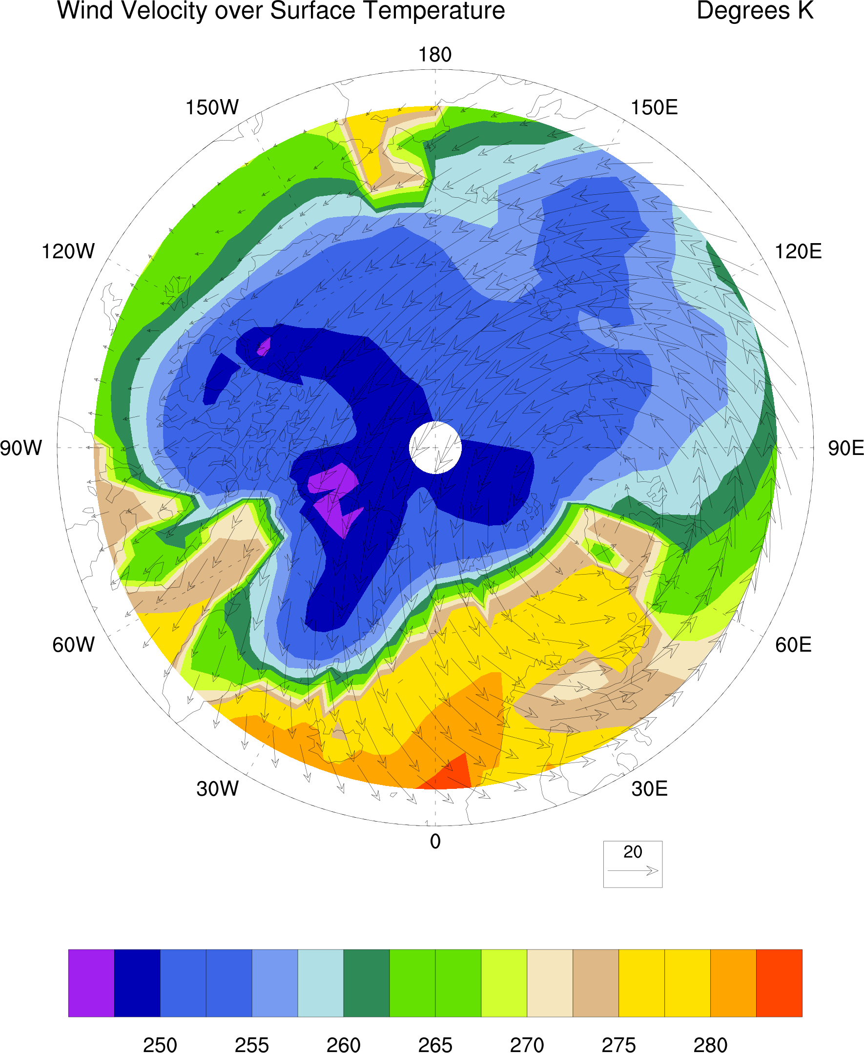
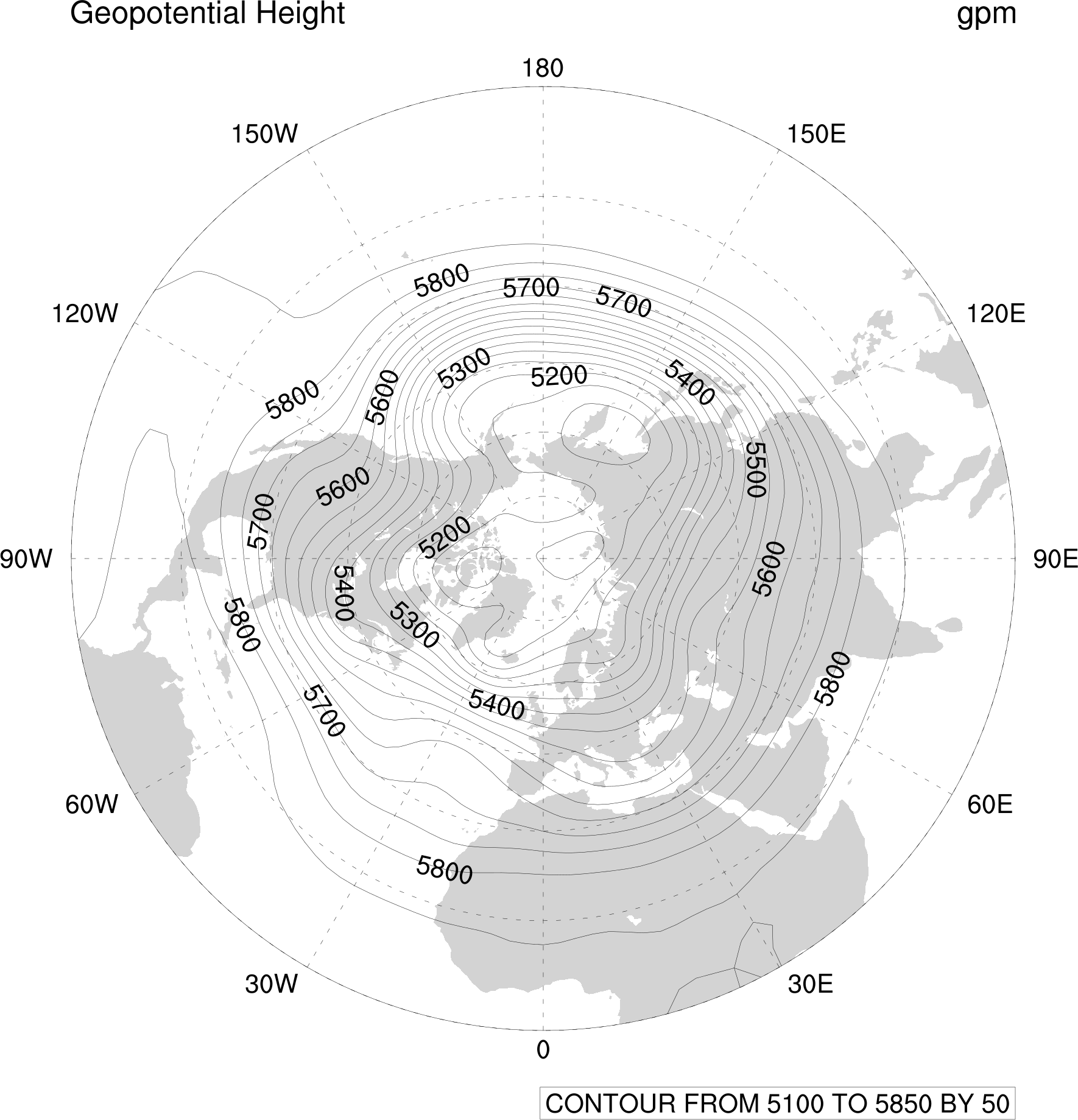
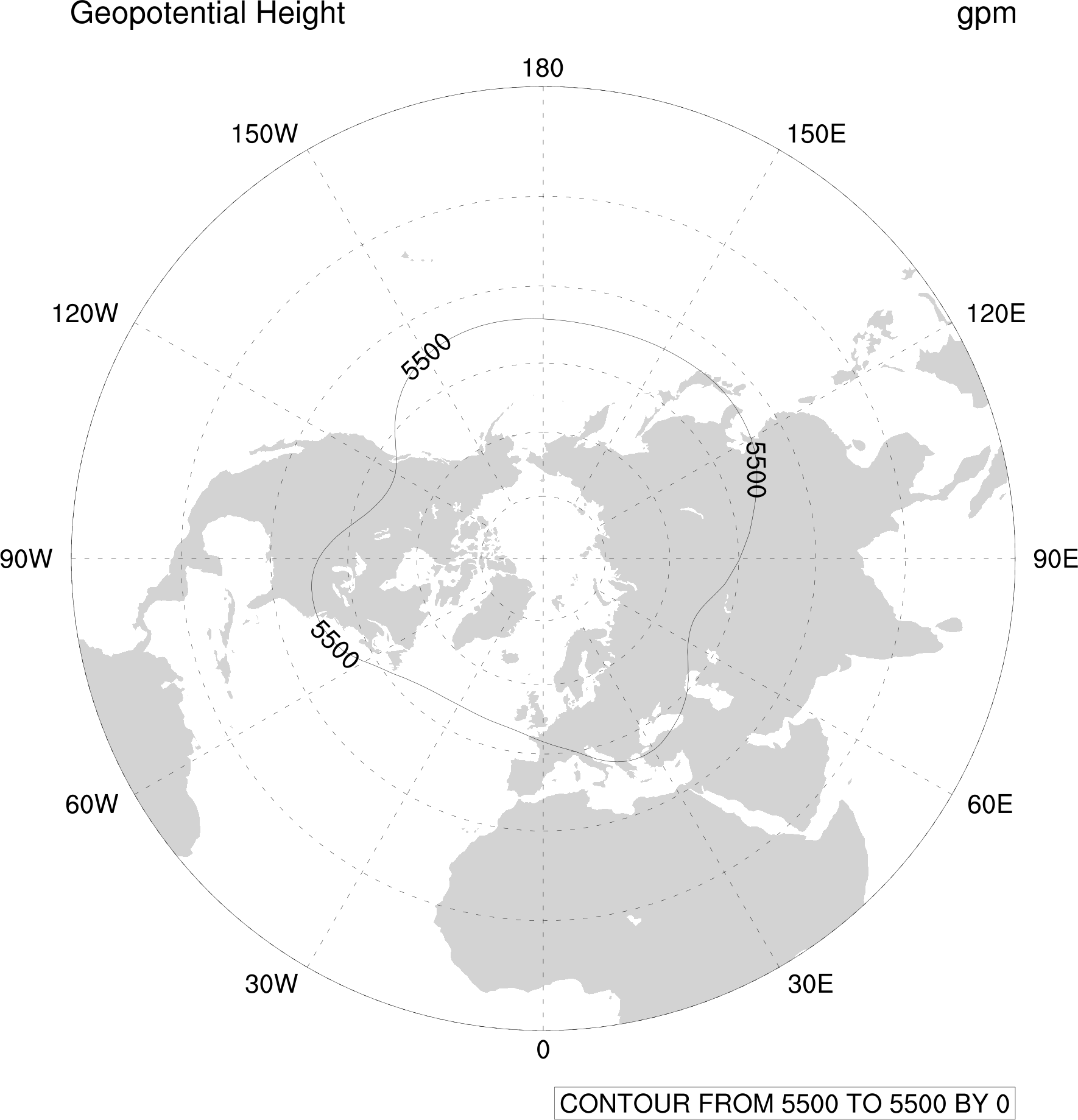
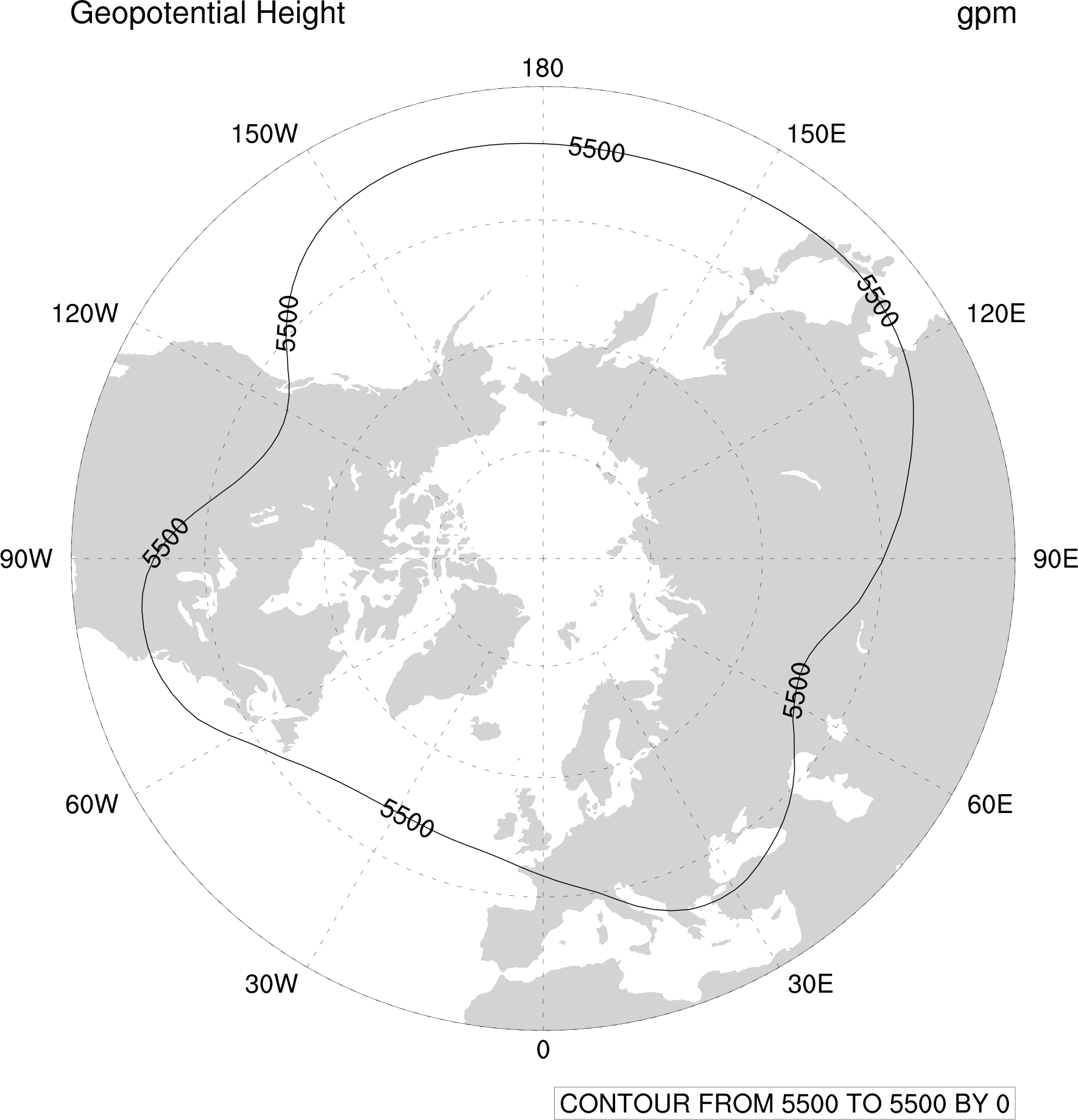
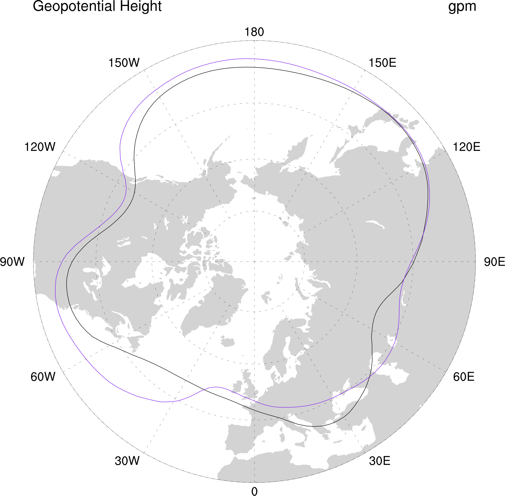
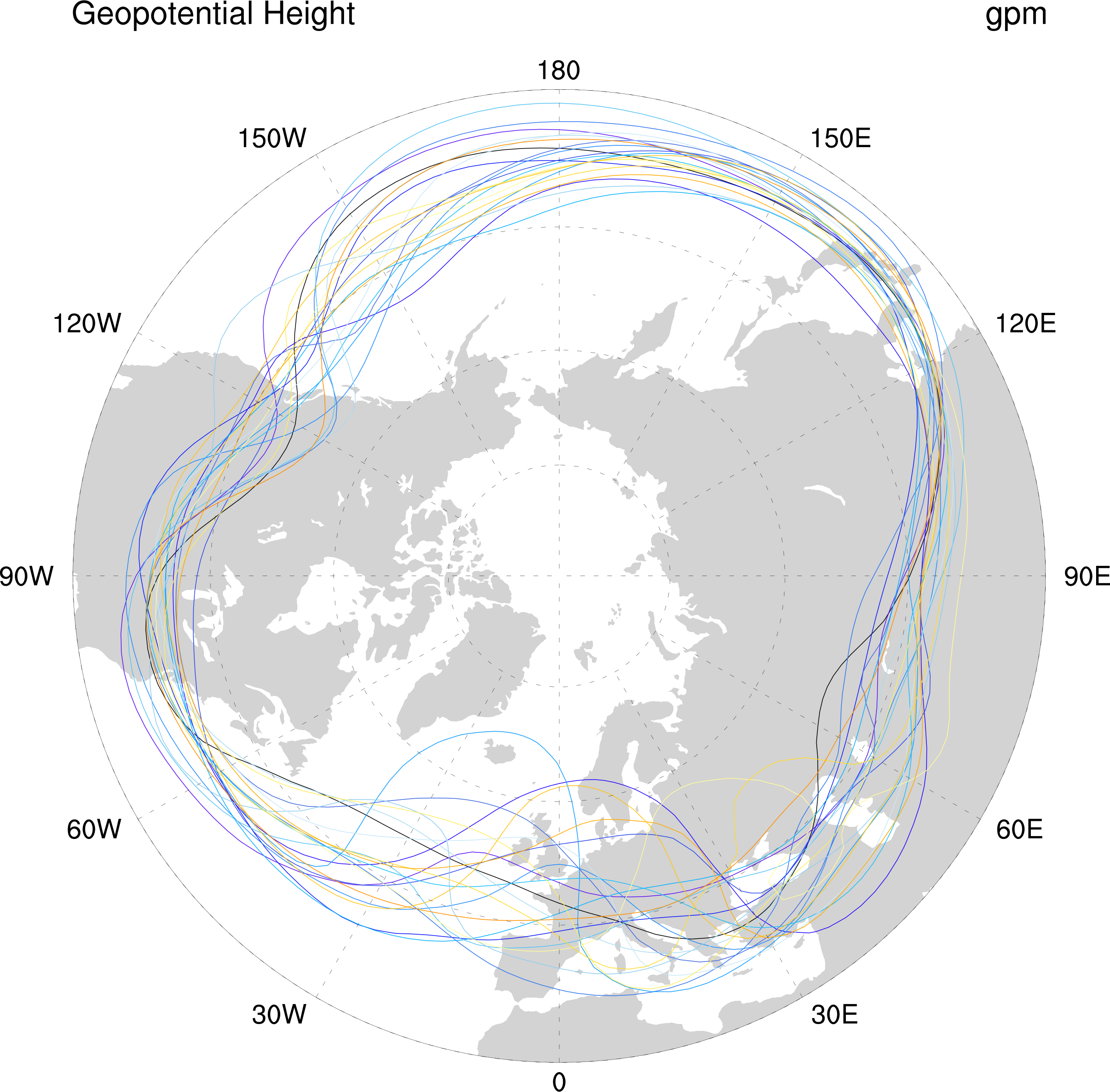
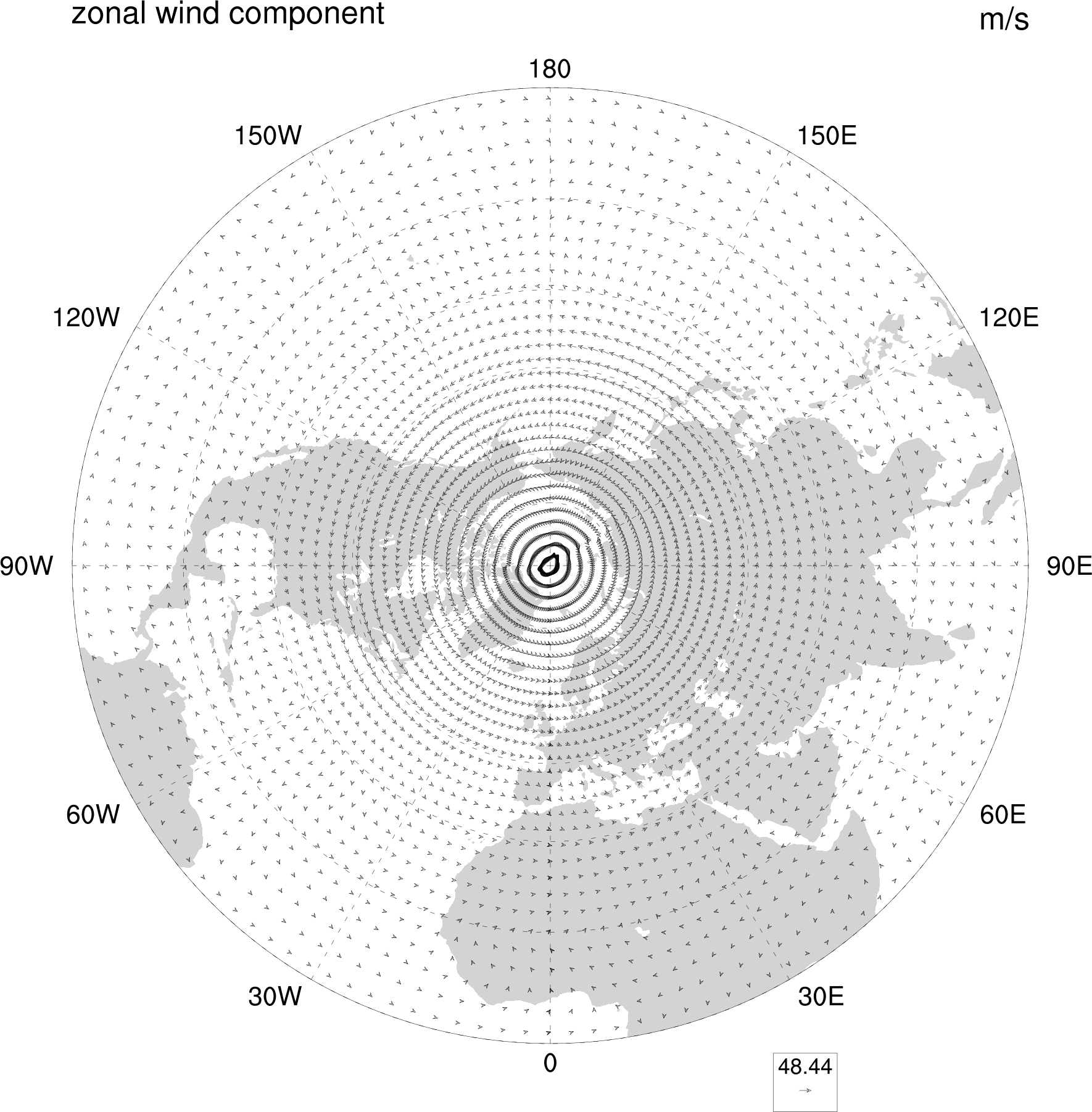
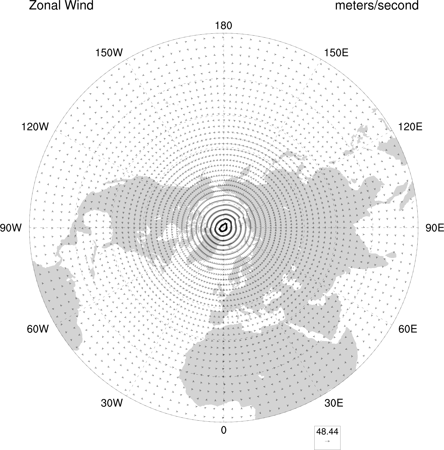
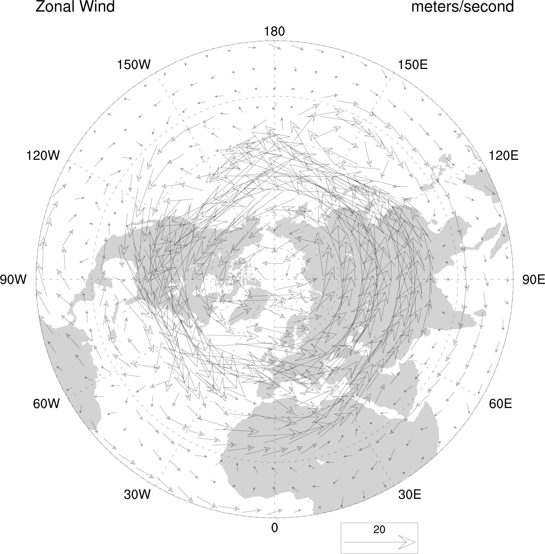
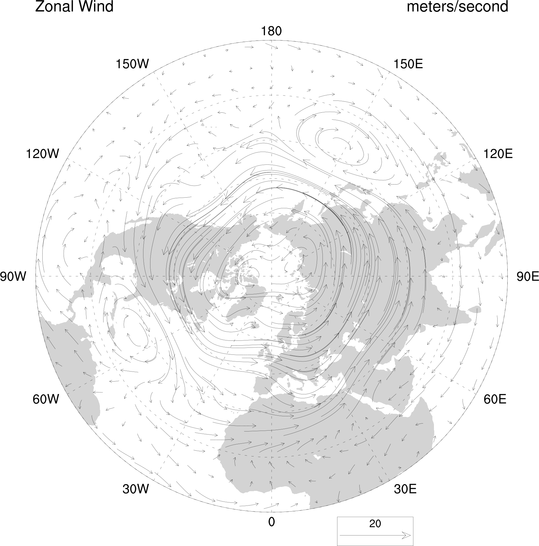
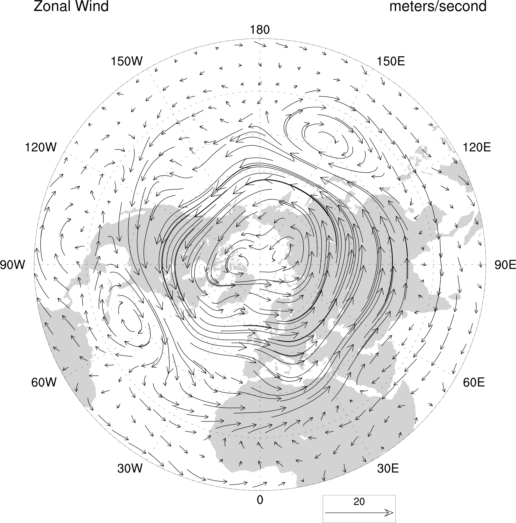
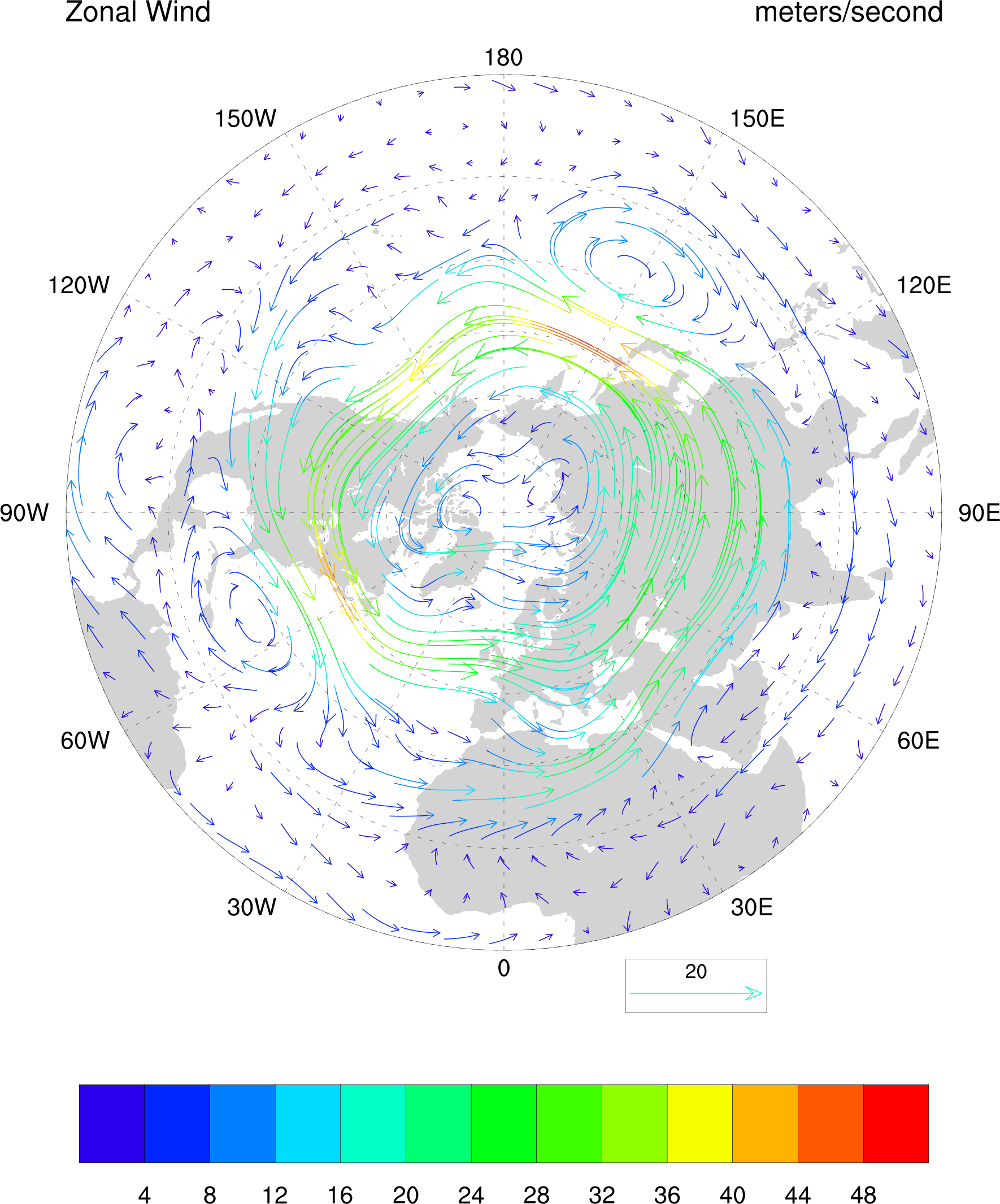
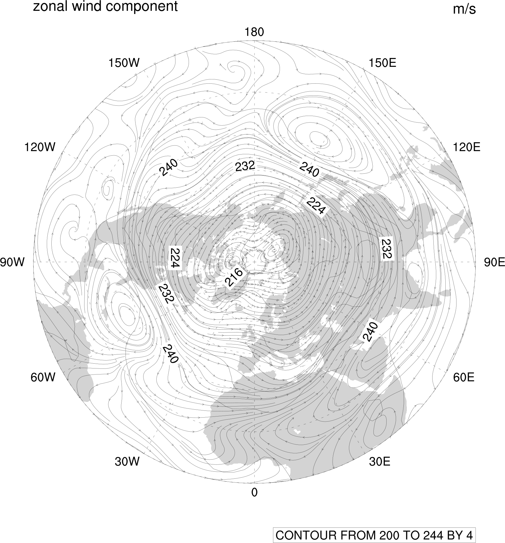
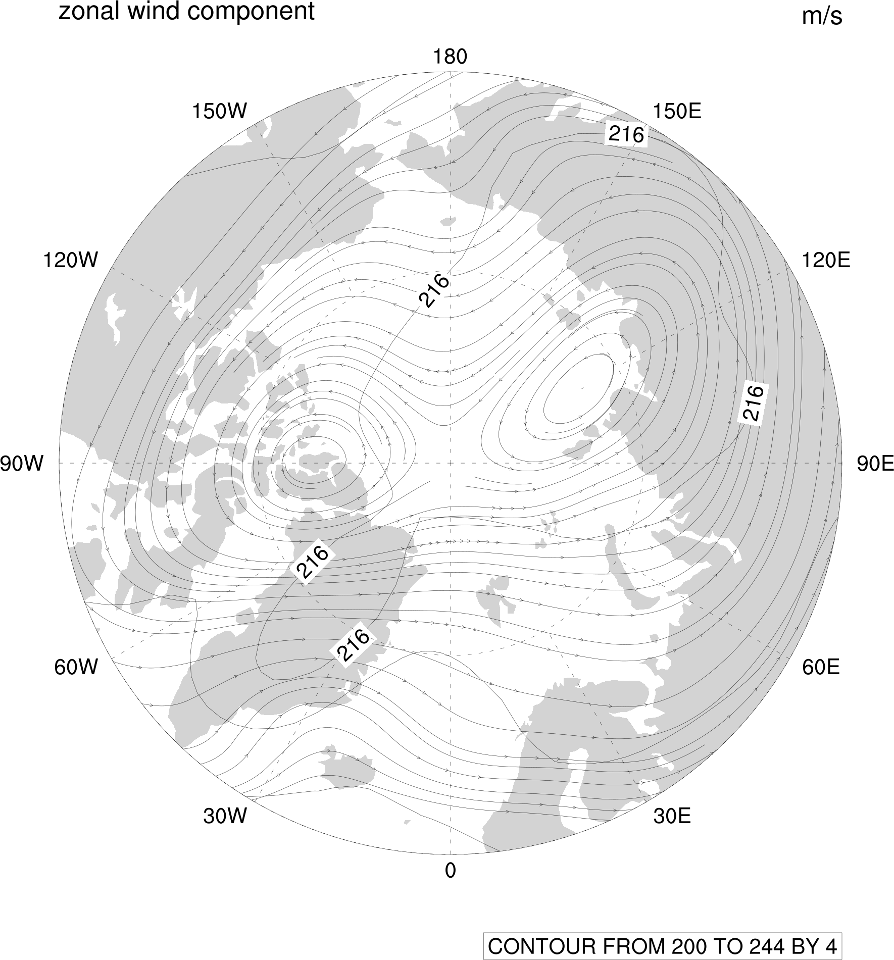
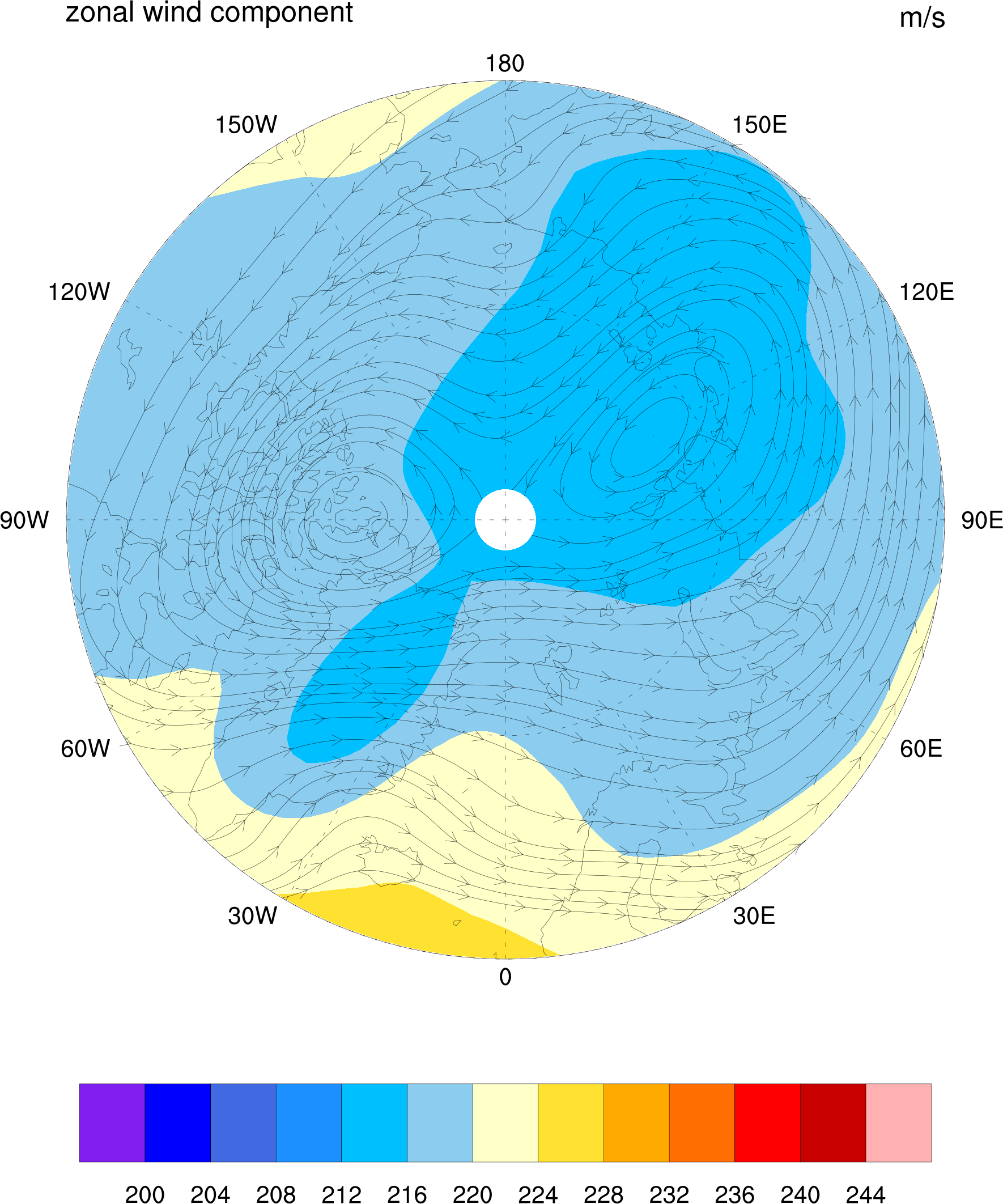
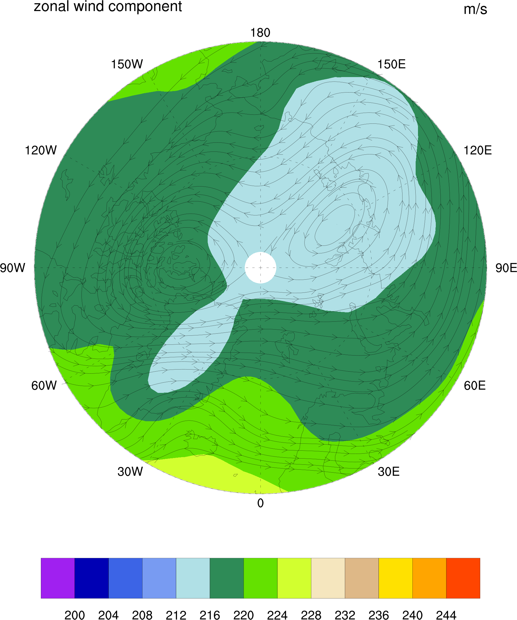
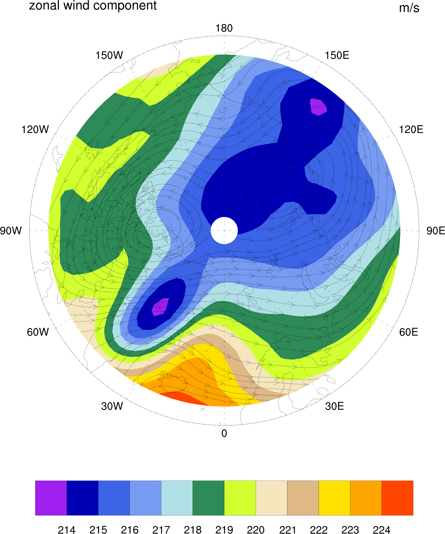
contours, vectors, or streamlines over polar stereographic page
|
| 
| 
| 
|
| ice.ncl | contour3j.ncl | contour3e.ncl | vector2g.ncl |
| |||
| stream1i.ncl |
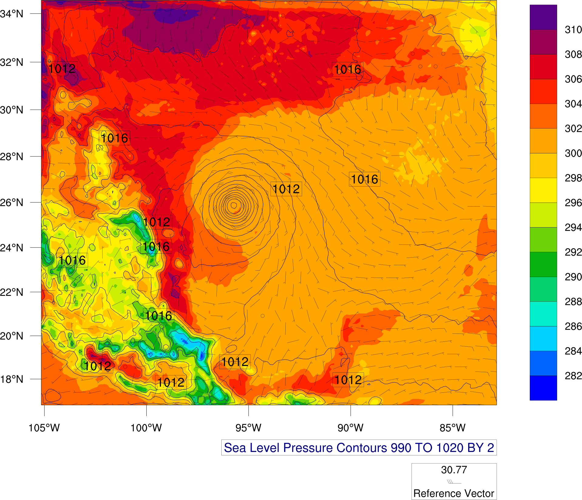
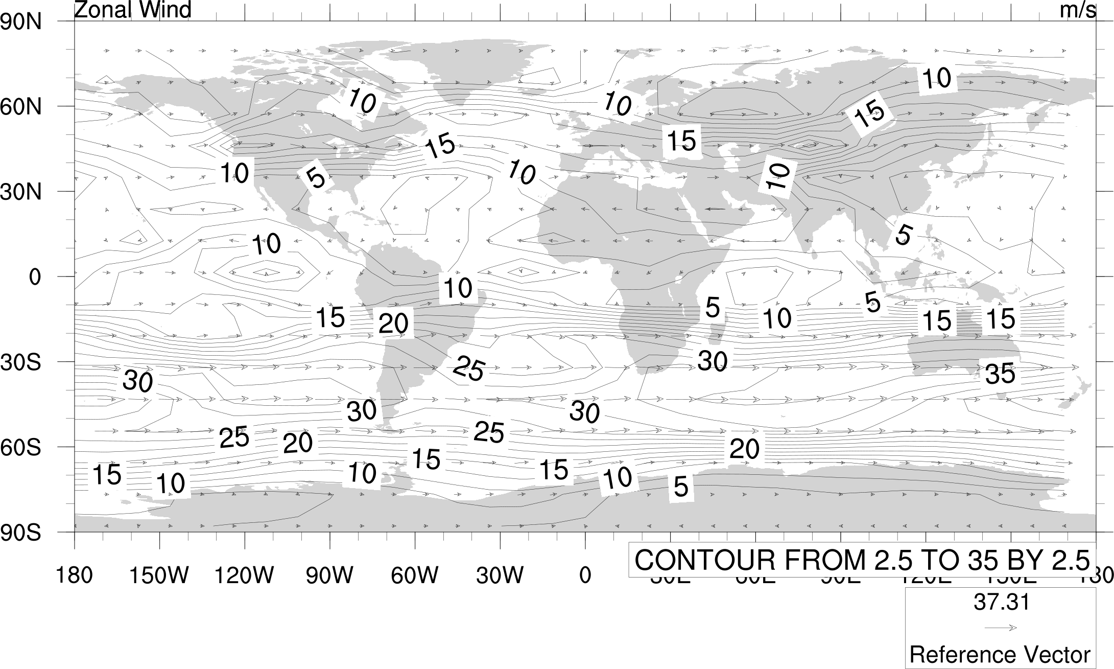
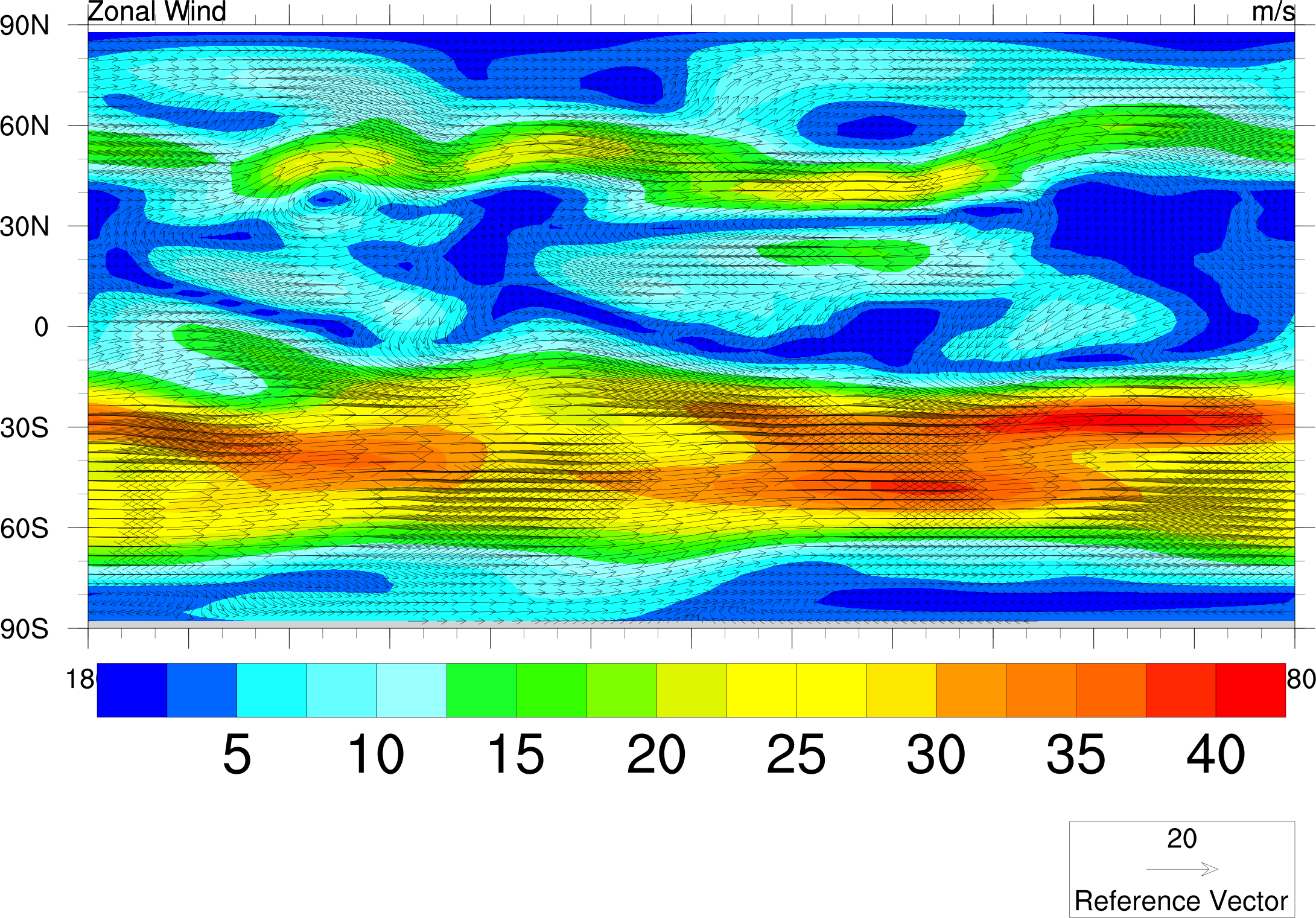
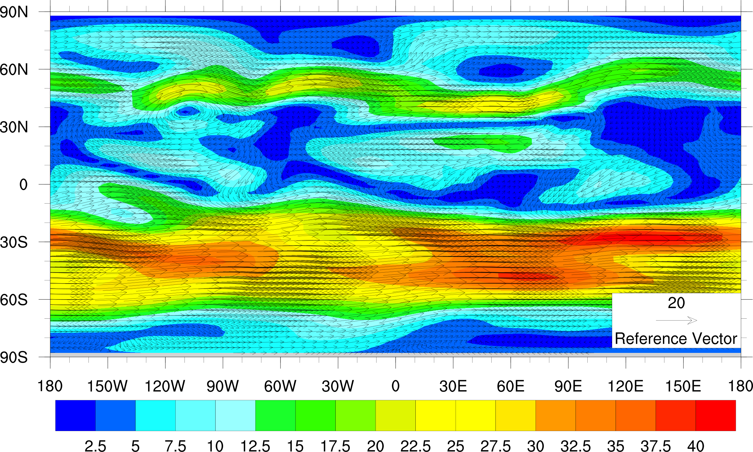
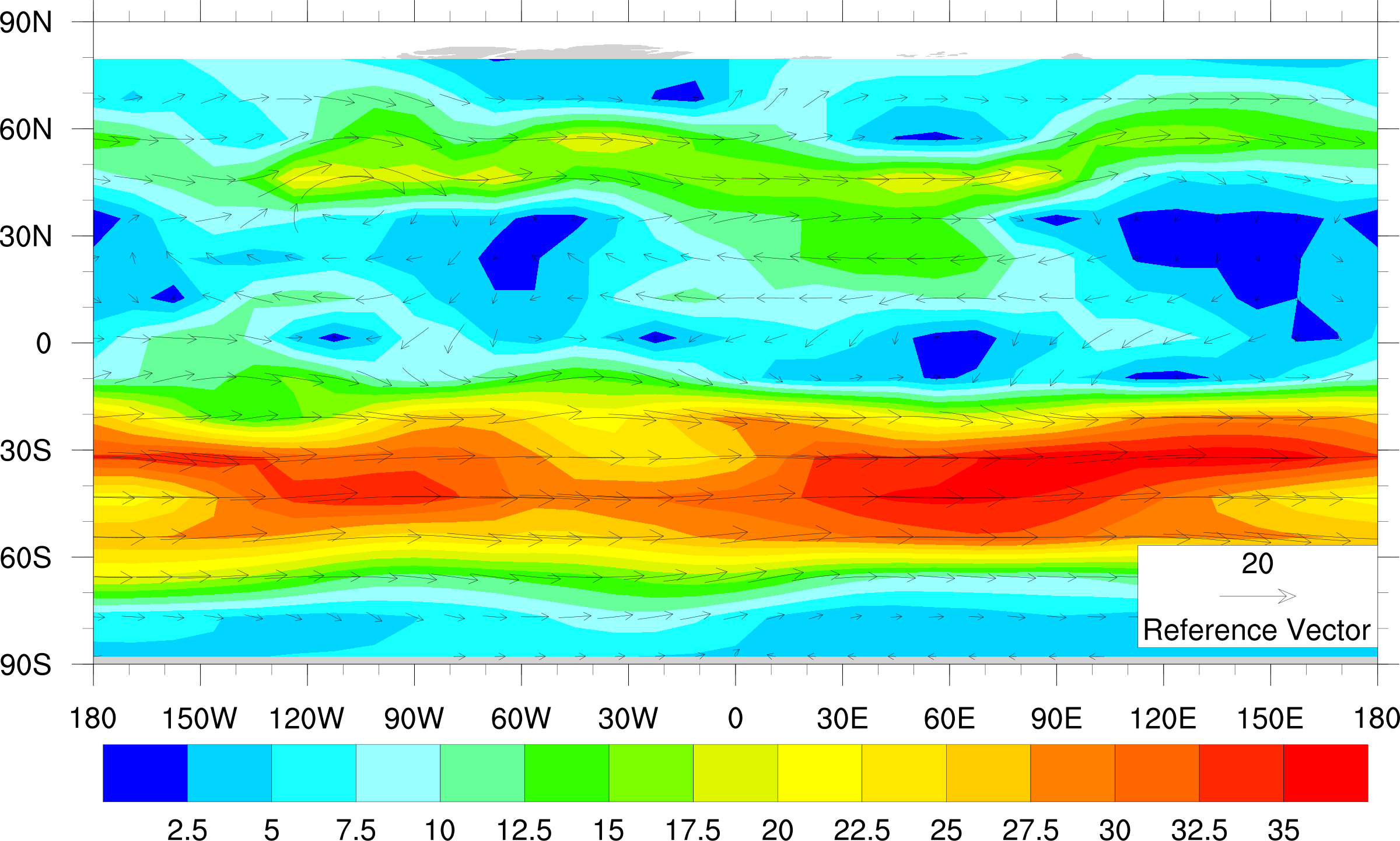
contours, vectors, streamlines over maps


function codes
| 
|
| fcodes.ncl | heart.ncl |
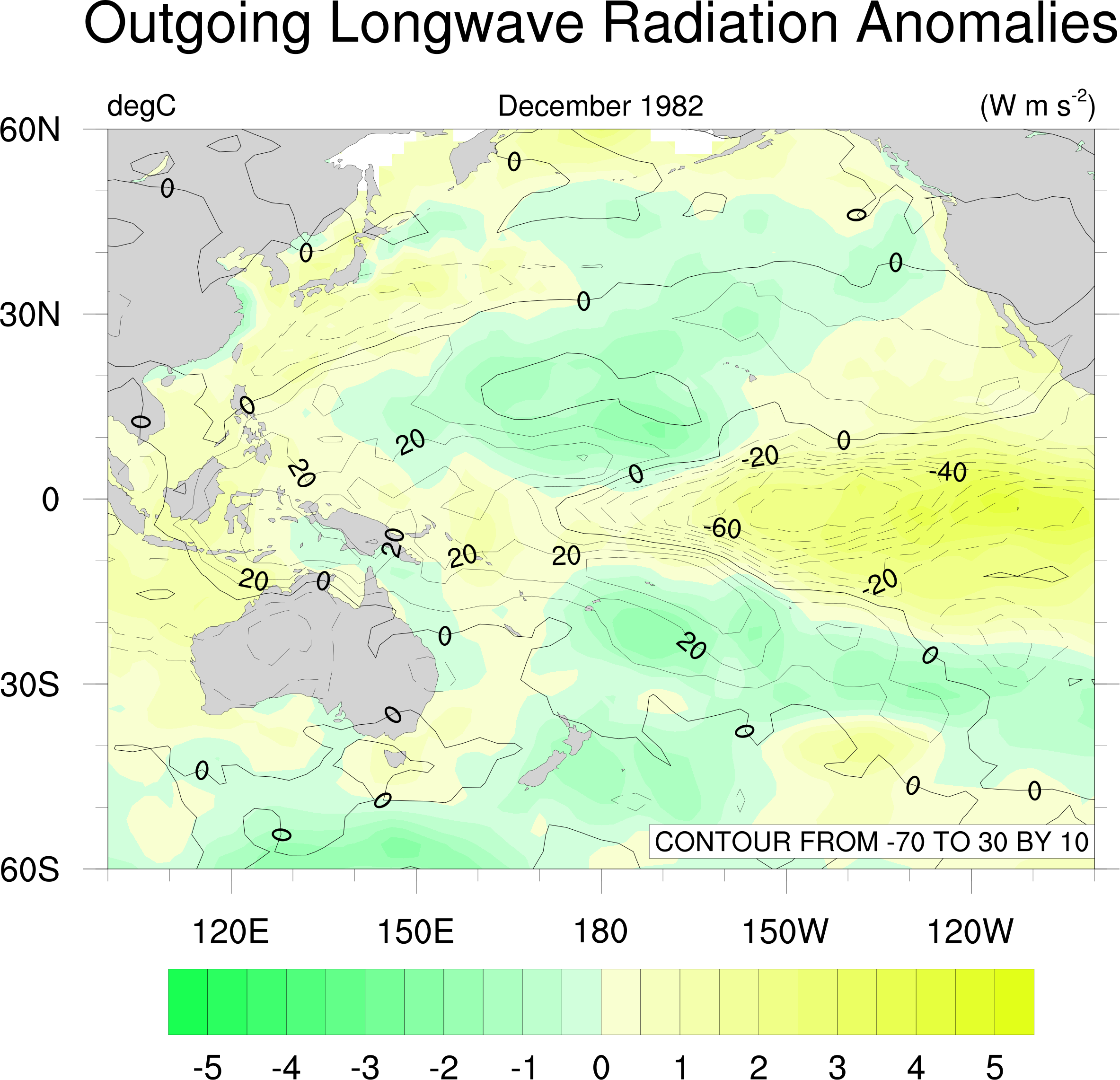
line contours over filled contours
|
| 
| 
| 
|
| contour9a.ncl | contour9b.ncl | contour9c.ncl | contour9d.ncl |
| 
| 
| |
| contour9e.ncl | contour9f.ncl | wrf_line_fill_vector_gsn.ncl |
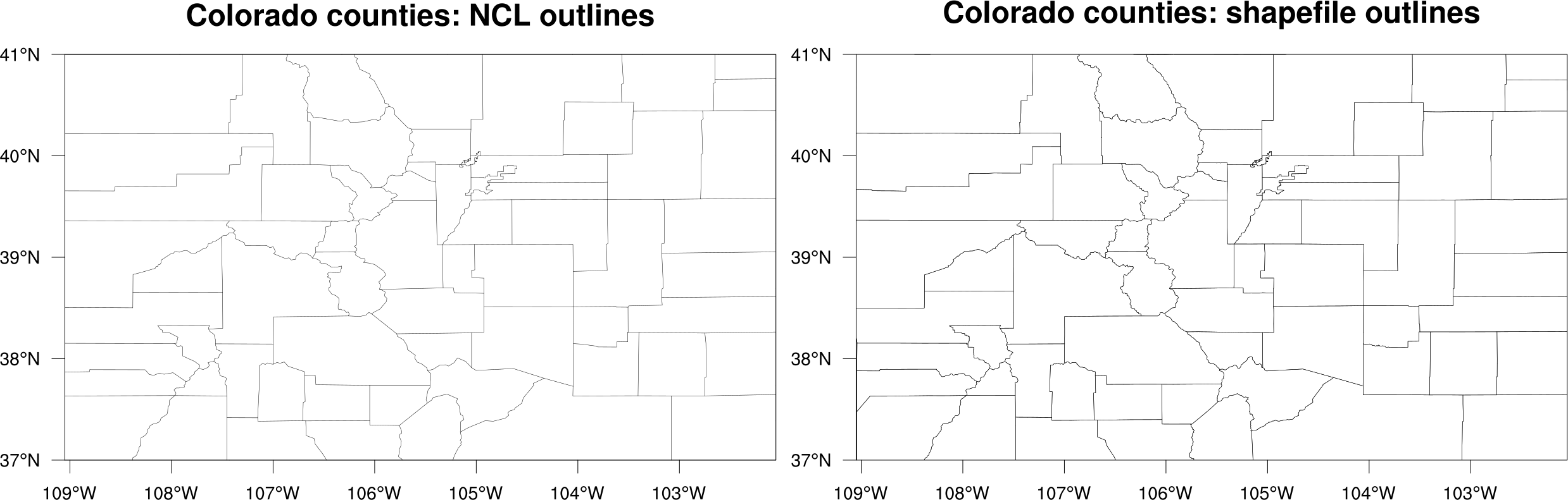
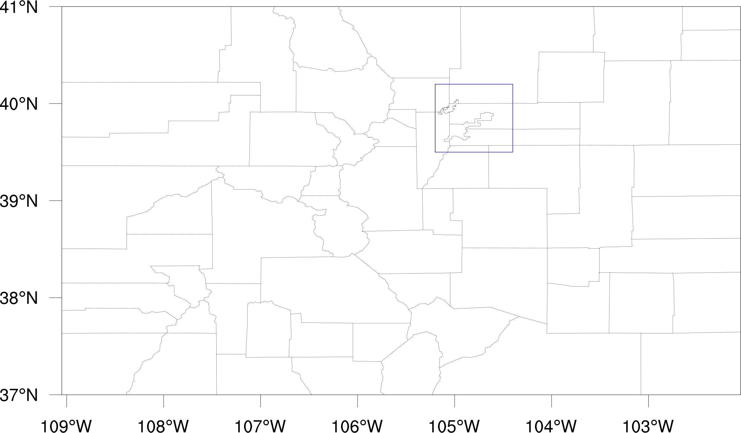
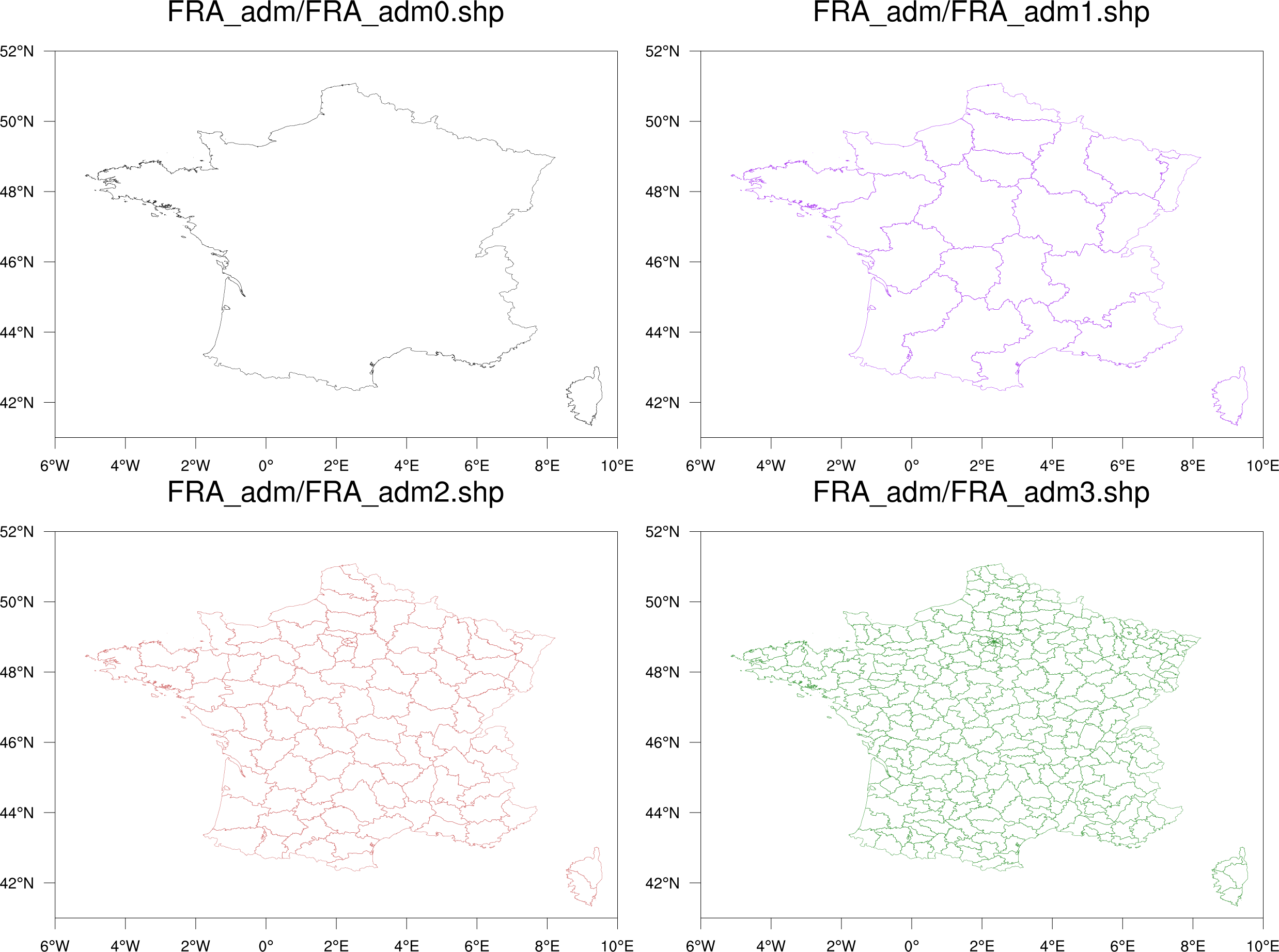
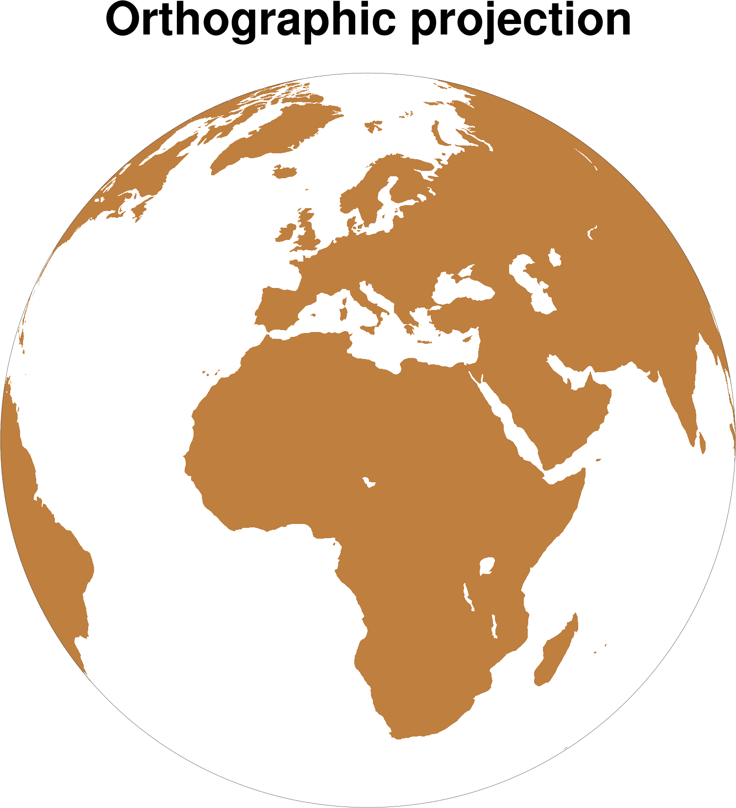
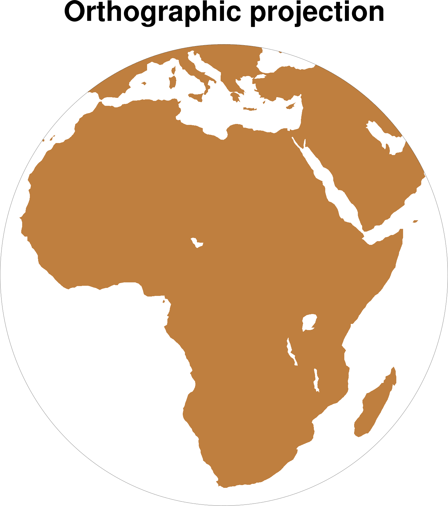
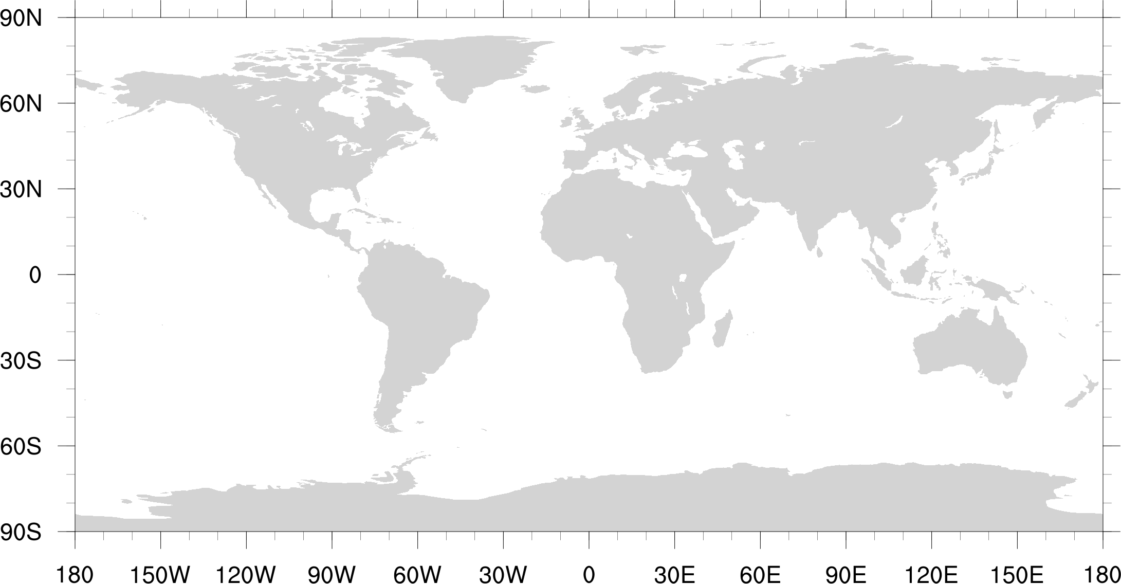
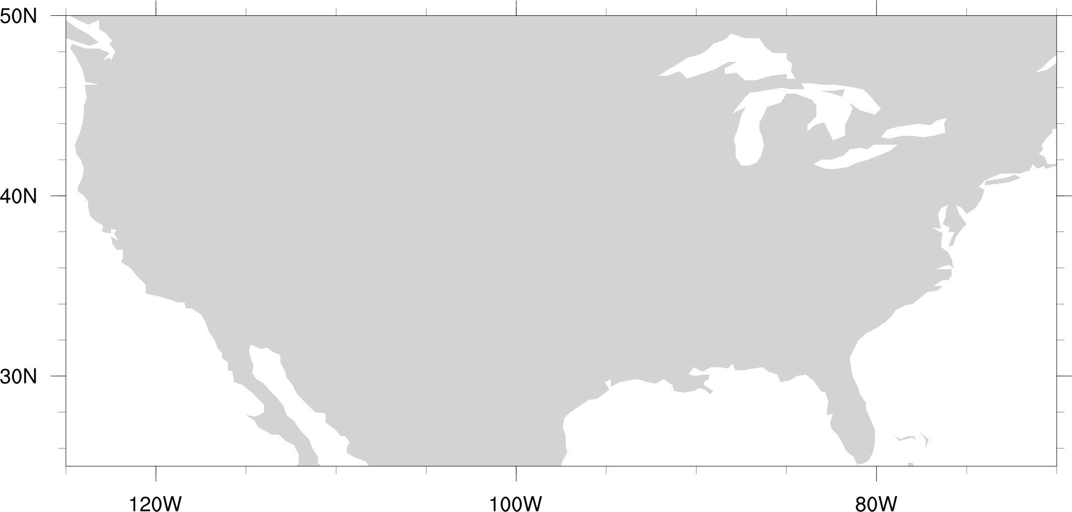
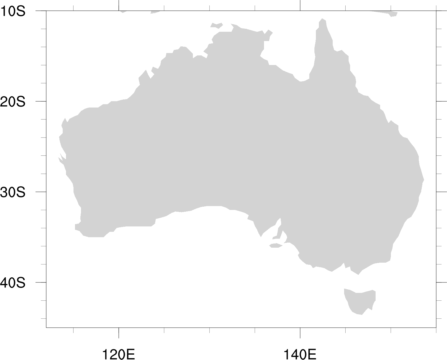
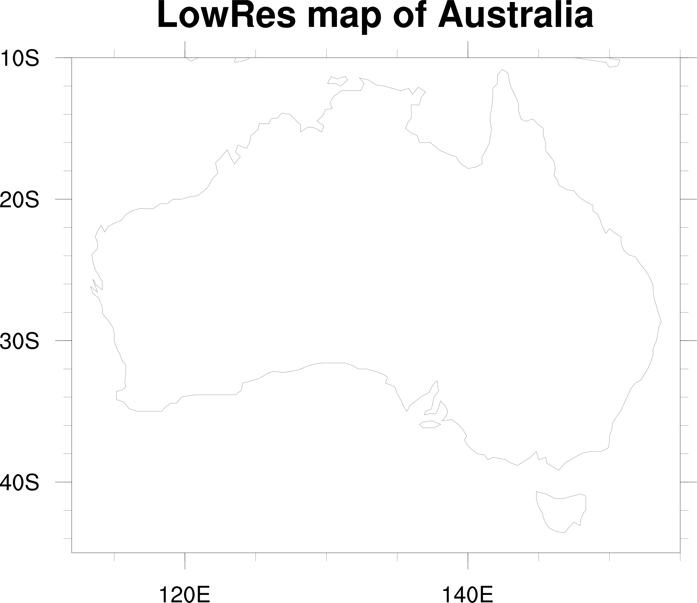
maps only
| 
| 
|
| colorado_map.ncl | colorado_map_640.ncl | france_shapefiles.ncl |
maximizing plots in frame
| 
| 
|
| max1a.ncl | max1b.ncl | max1c.ncl |
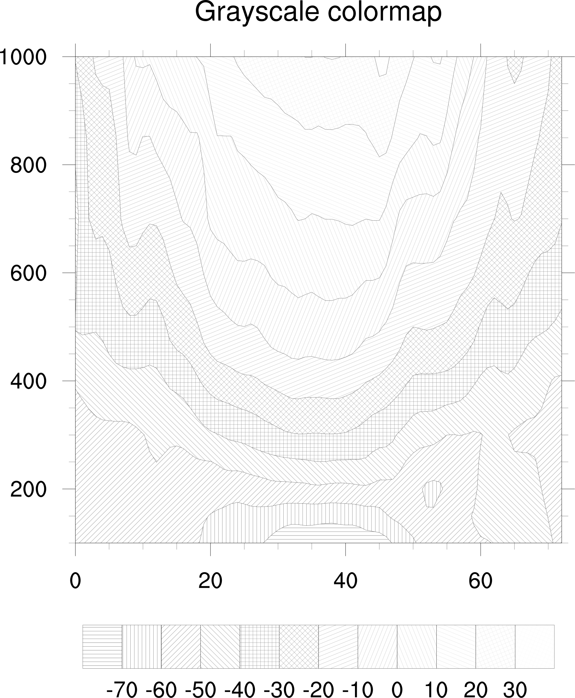
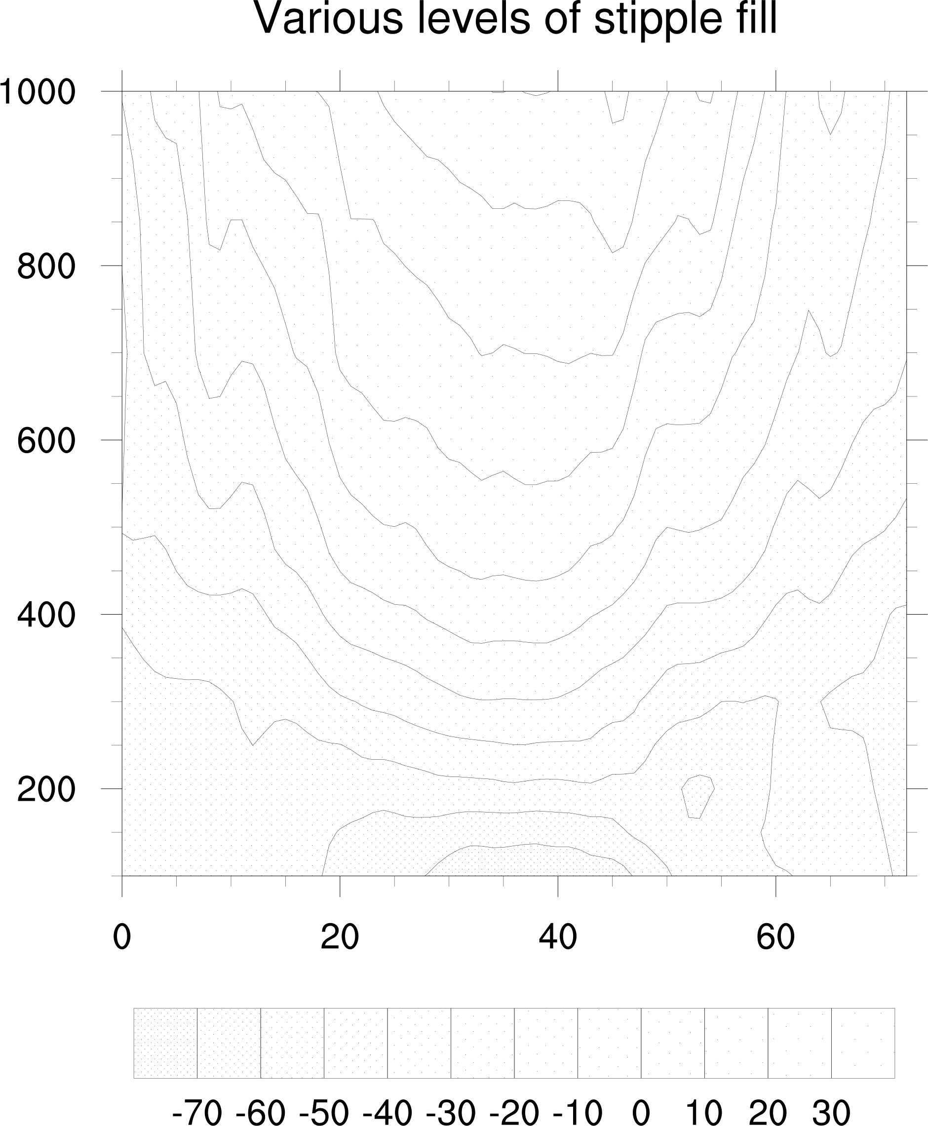
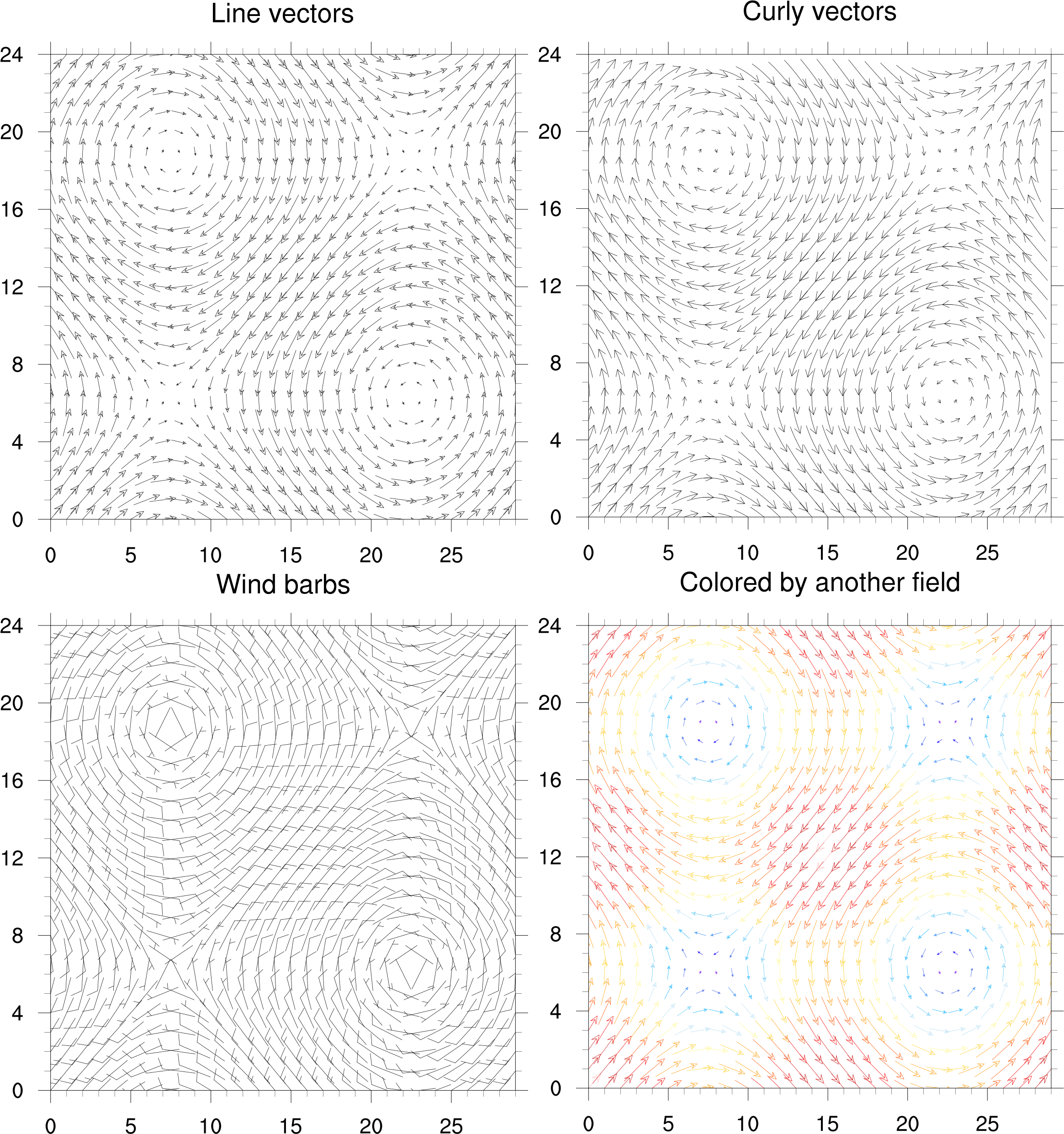
miscellaneous scripts
| 
| 
|
|
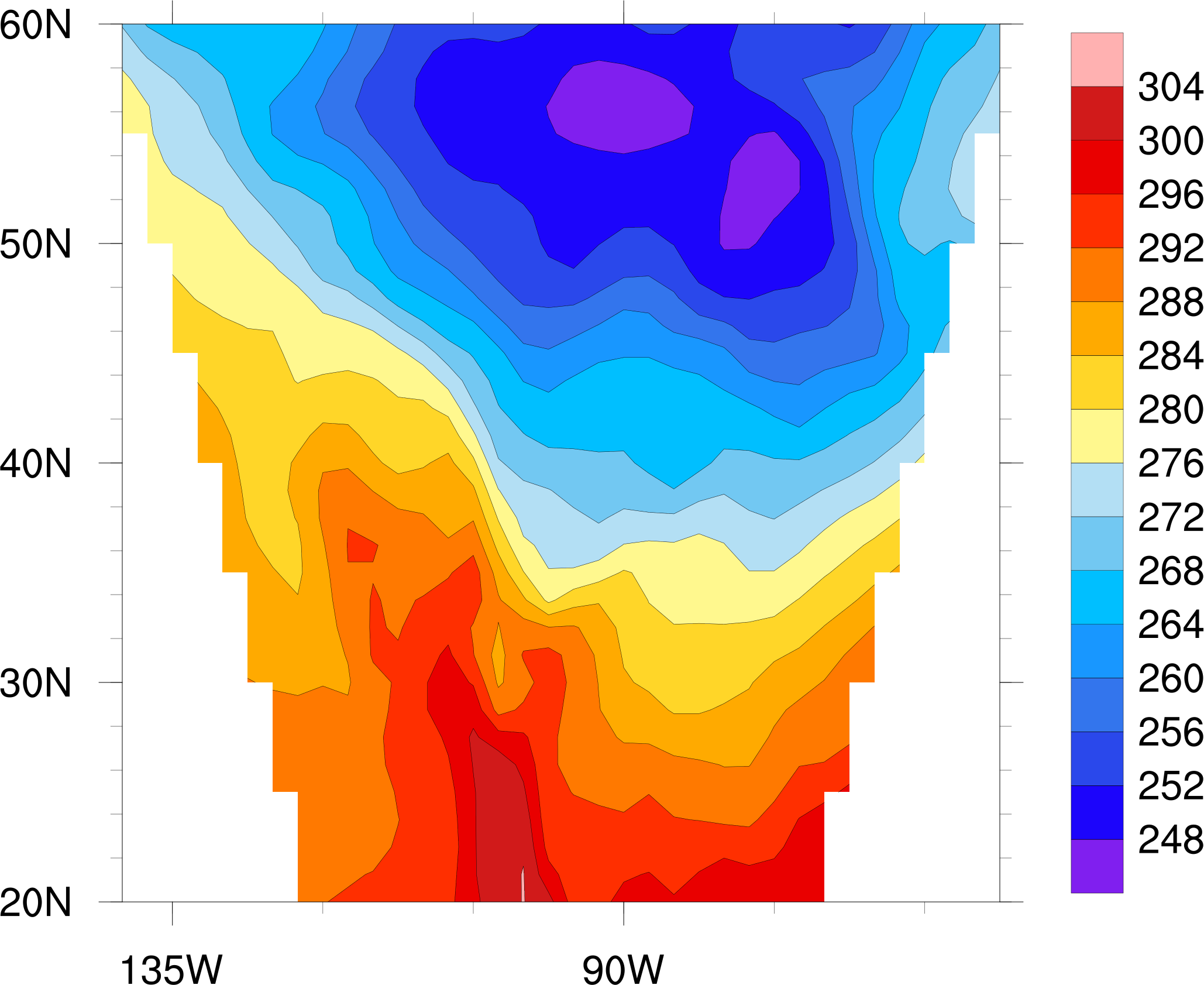
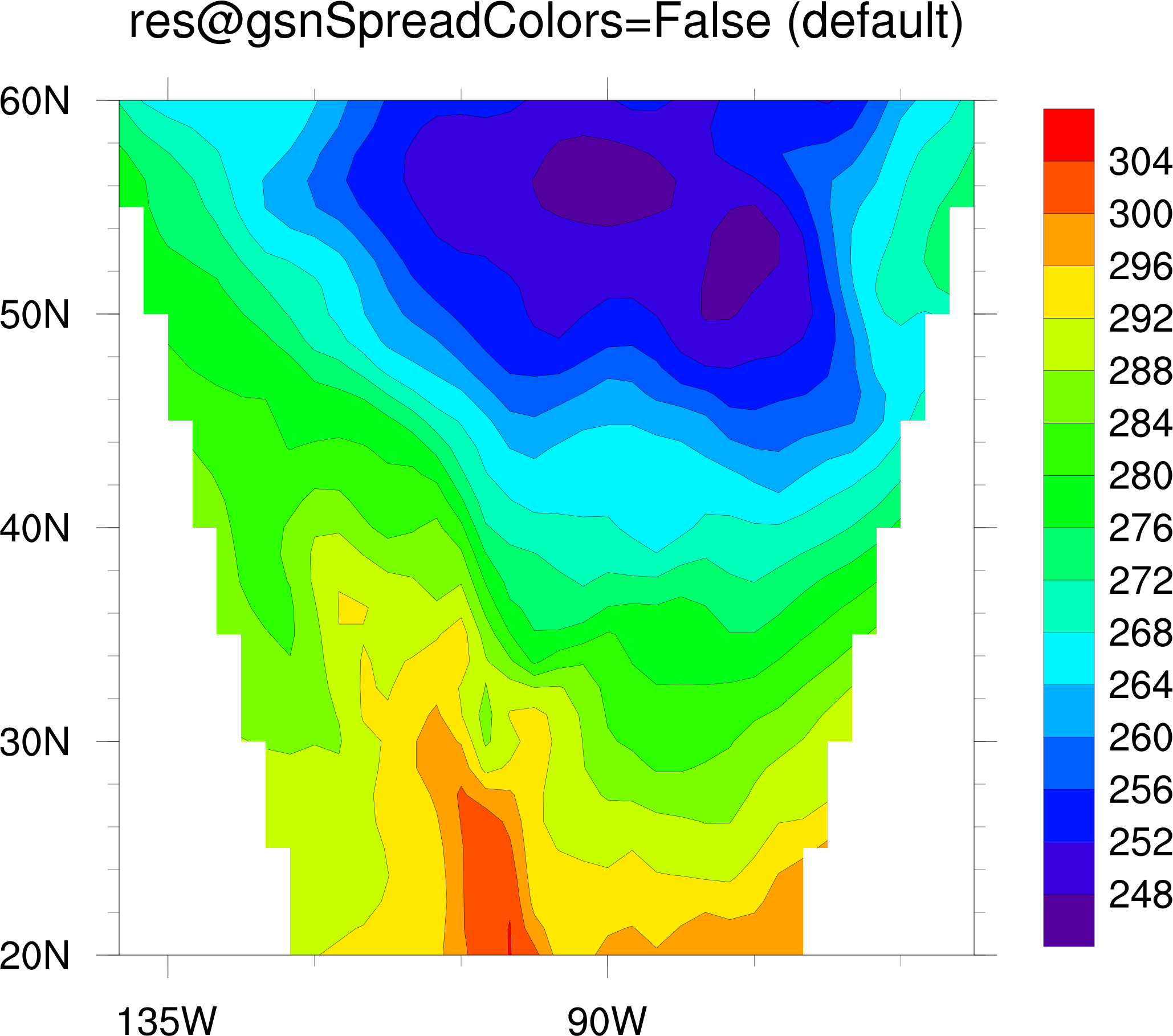
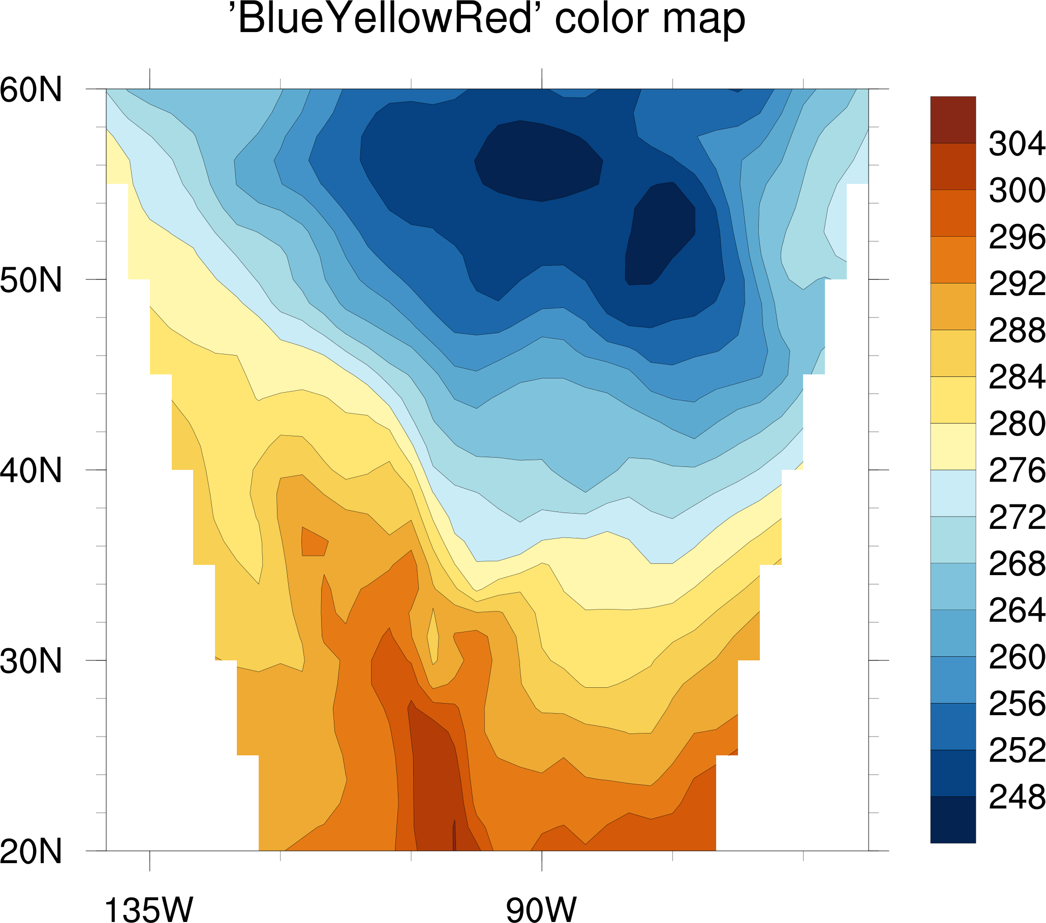
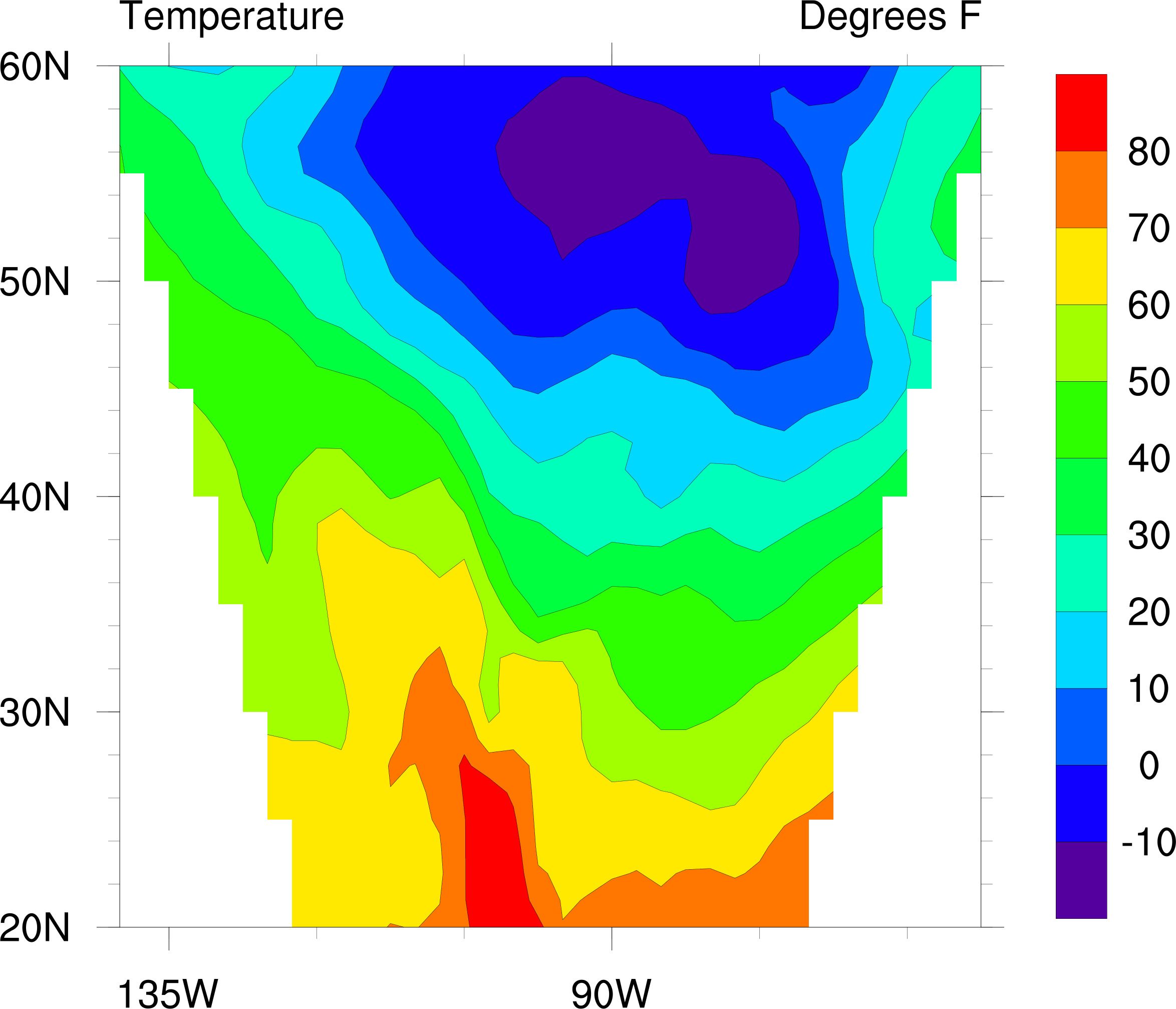
| compare_gsn_scripts.ncl | contour_color_tables.ncl | contour_fill_types.ncl | fcodes.ncl |
|
| 
| 
| 
|
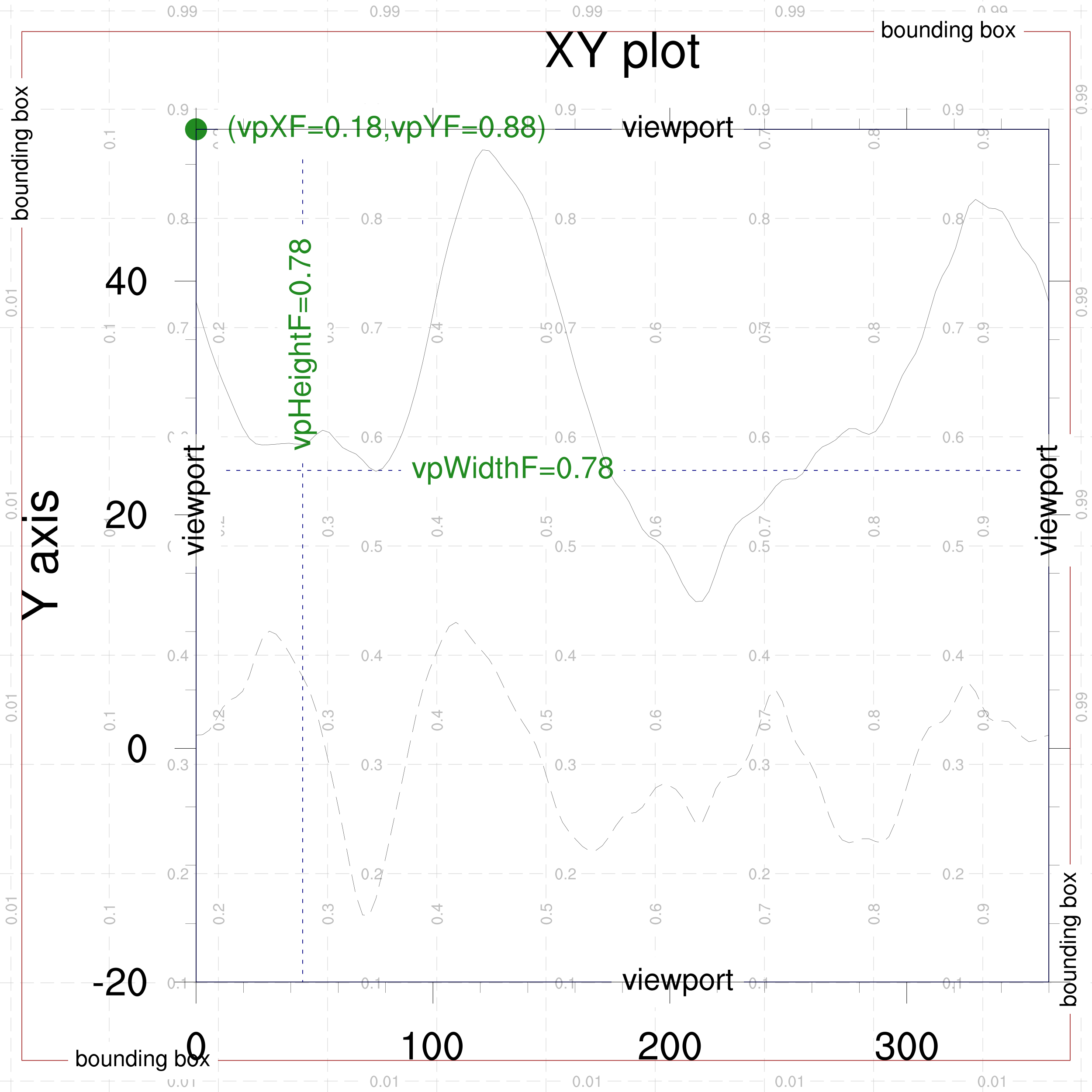
| heart.ncl | streamline_example.ncl | vector_types.ncl | viewport.ncl |

| 
| ||
| vp_frames.ncl | xy_a4.ncl |
multiple plots on a page
| 
| 
| 
|
| panel1a.ncl | panel1b.ncl | panel1c.ncl | panel1d.ncl |
| 
| 
| 
|
| panel1e.ncl | panel1f.ncl | panel1g.ncl | panel1h.ncl |
| 
| 
| 
|
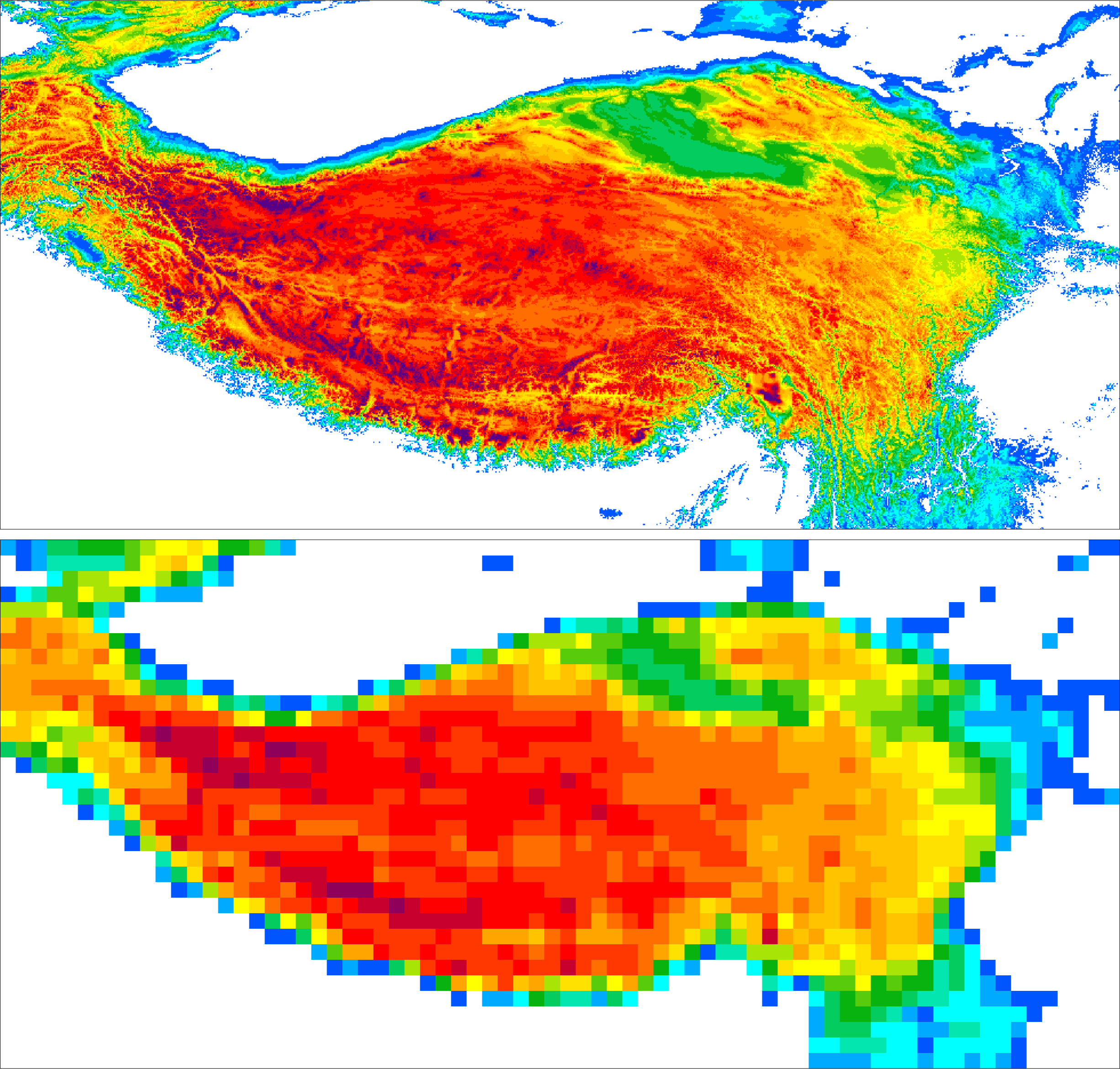
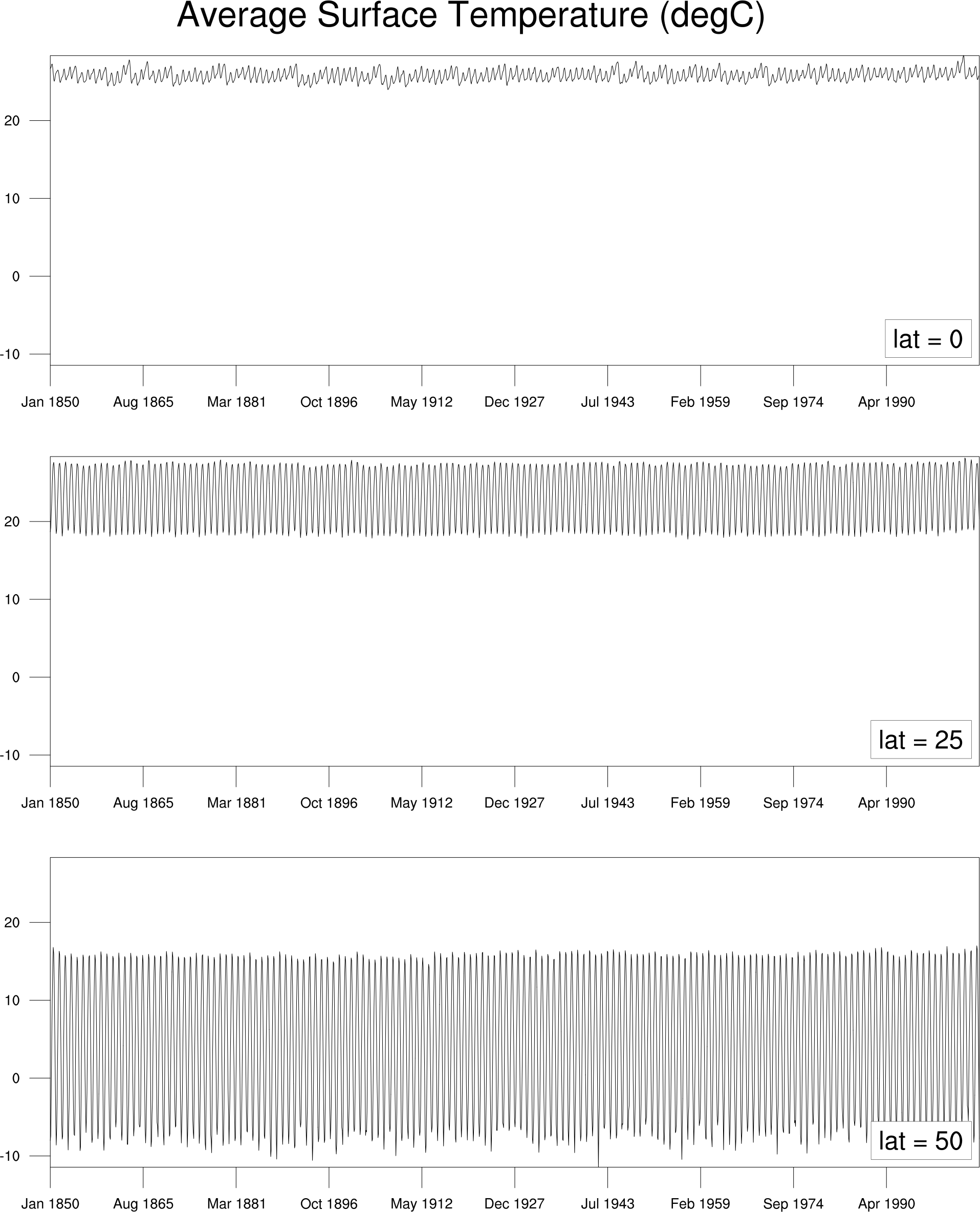
| panel1i.ncl | panel1j.ncl | tibet.ncl | time1h.ncl |
|
| 
| 
| |
| france_shapefiles.ncl | overlay_subset.ncl | xy_stacked.ncl |
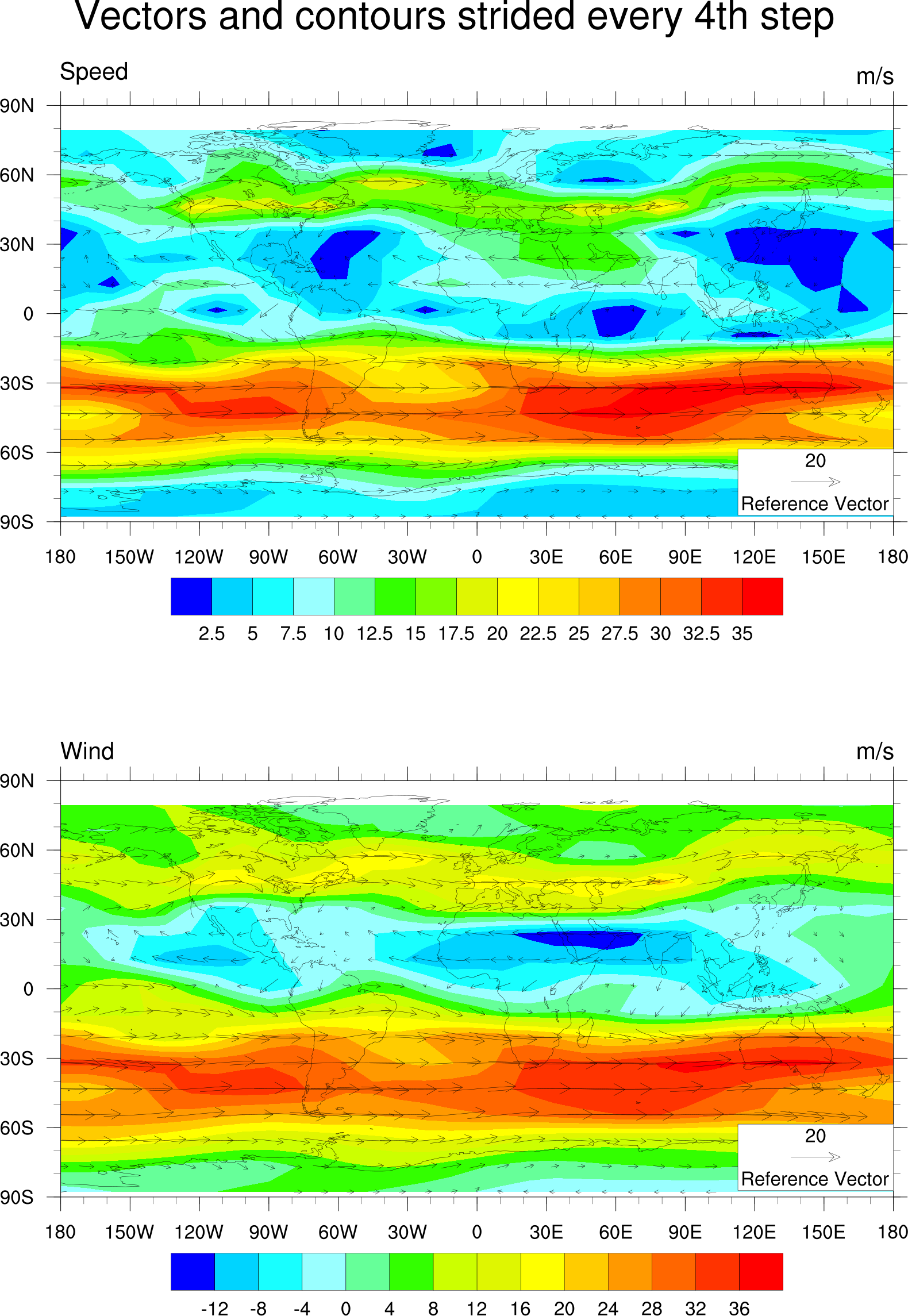
overlaying multiple fields on a map

| 
| 
| 
|
| overlay1a.ncl | overlay1b.ncl | overlay1c.ncl | overlay1d.ncl |
|
| ||
| overlay1e.ncl | wrf_line_fill_vector_gsn.ncl |
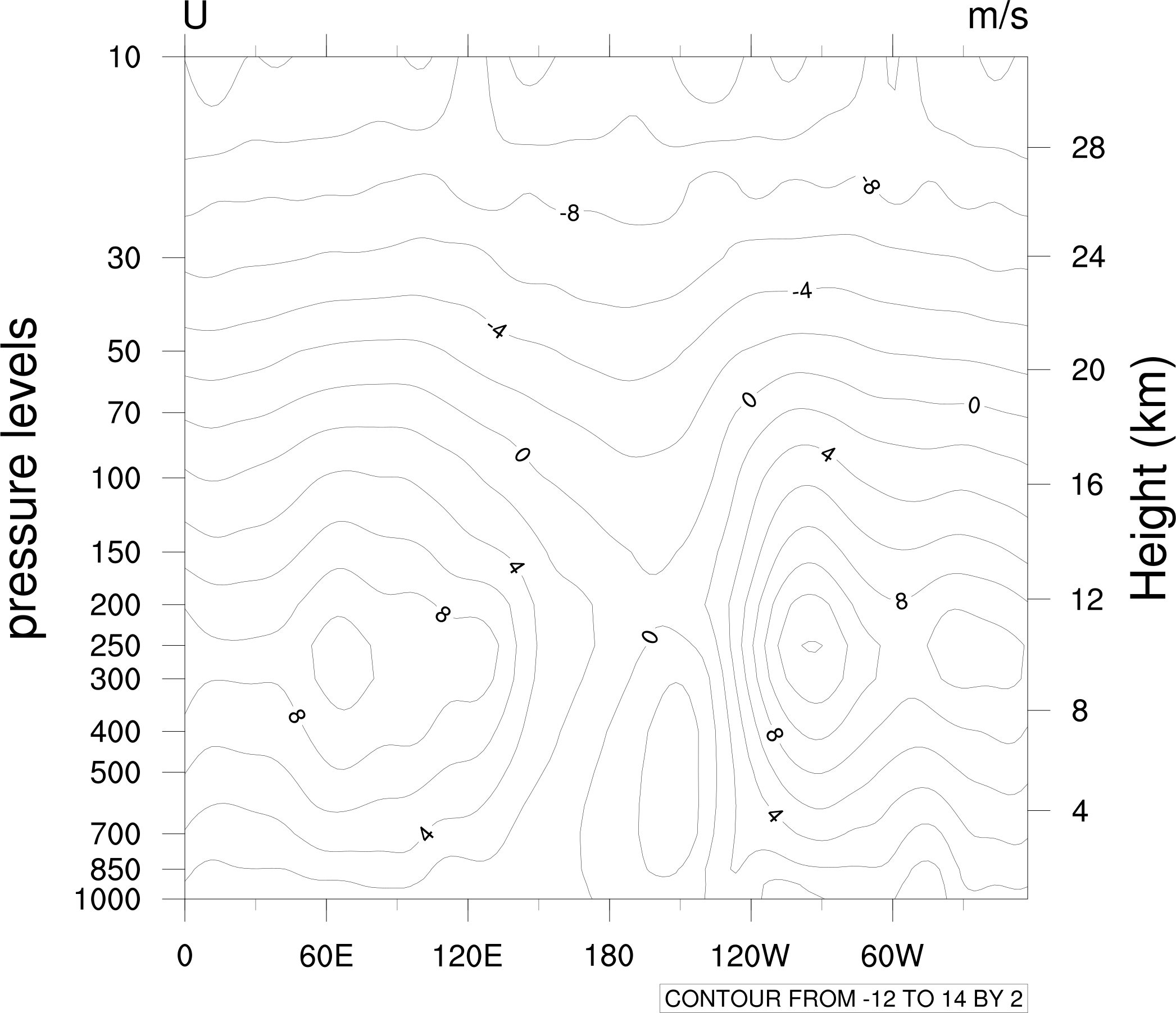
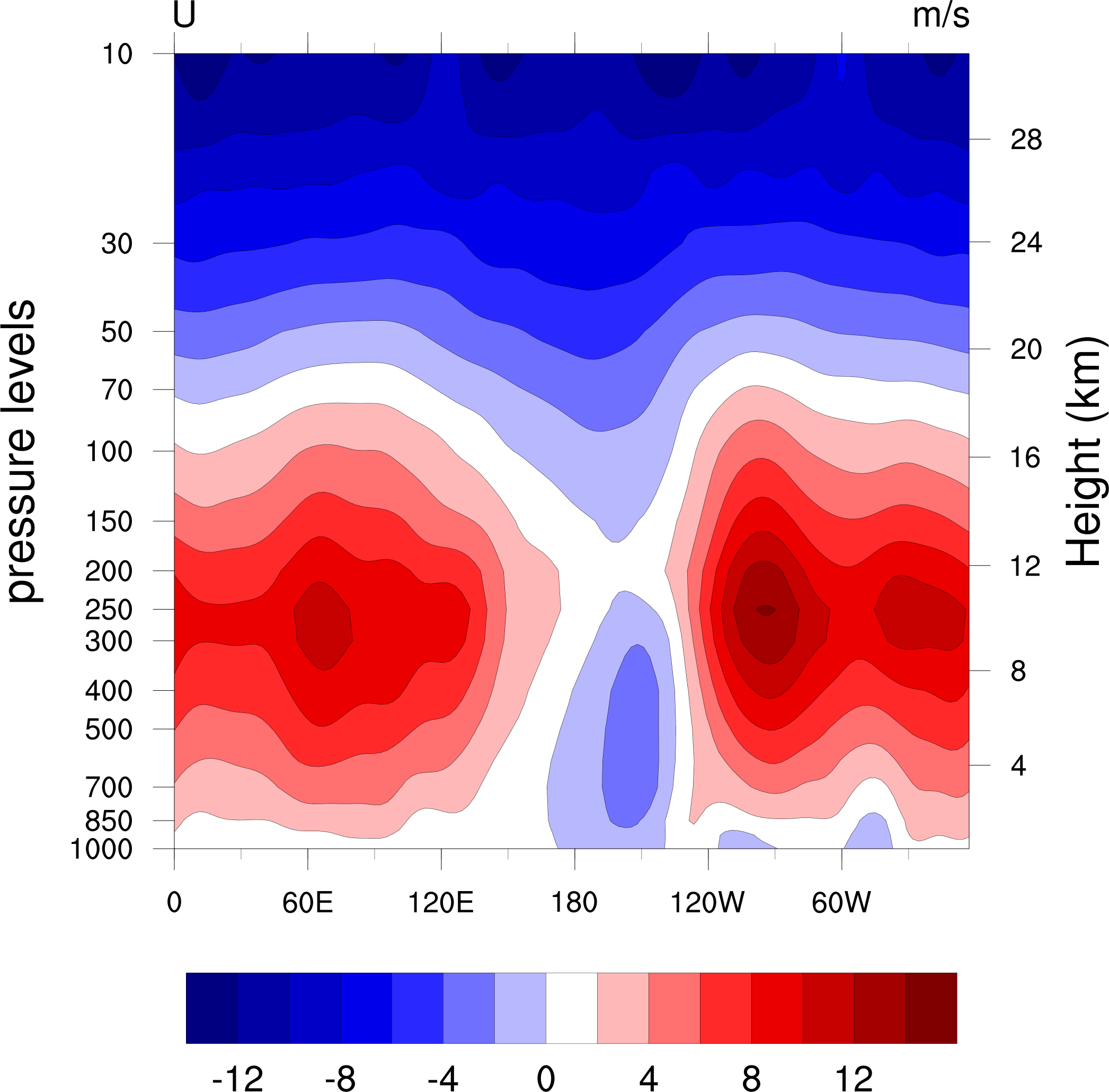
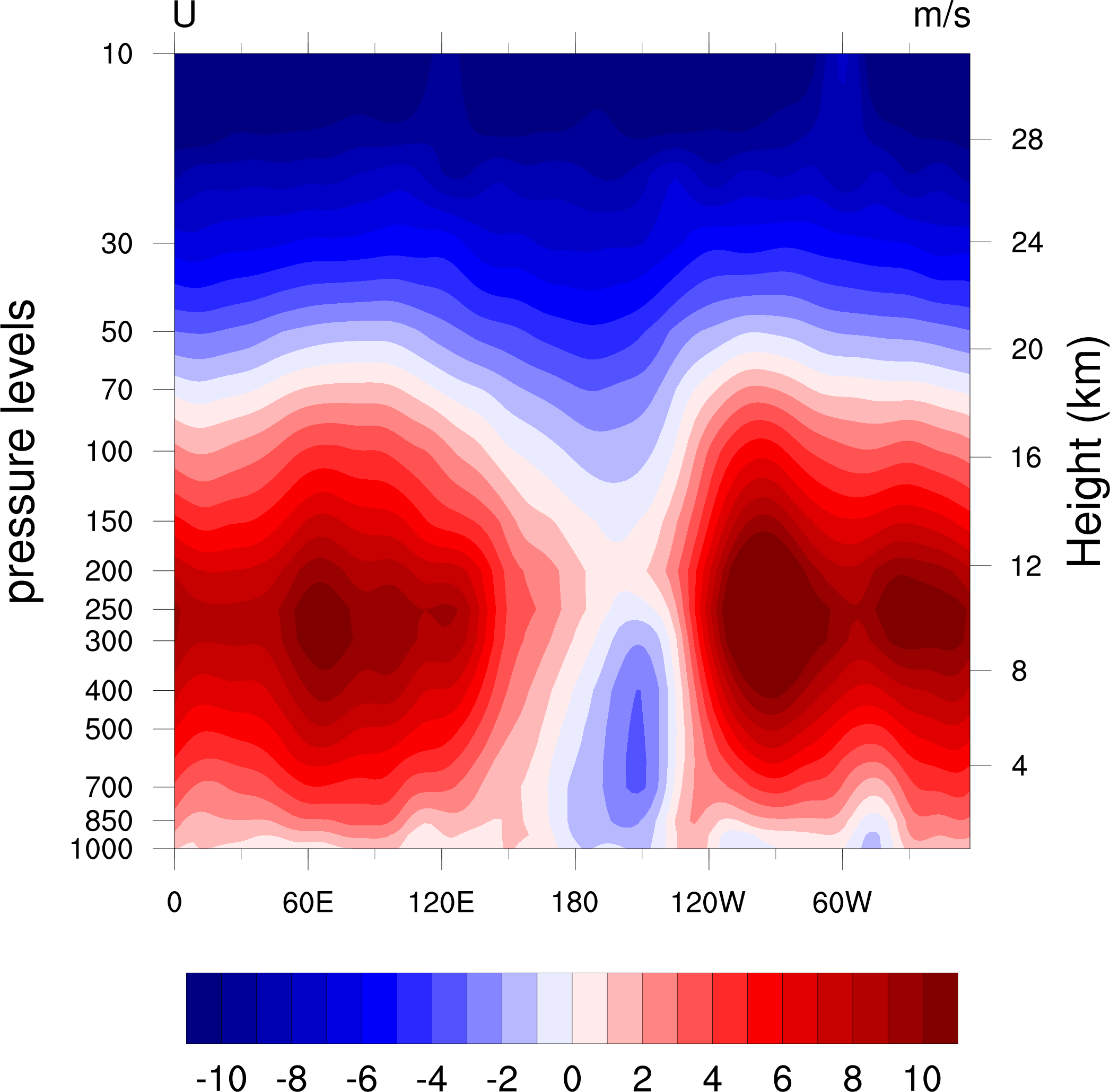
pressure/height plots
| 
| 
| 
|
| preshgt1a.ncl | preshgt1b.ncl | preshgt1c.ncl | preshgt1d.ncl |

| |||
| preshgt1e.ncl |
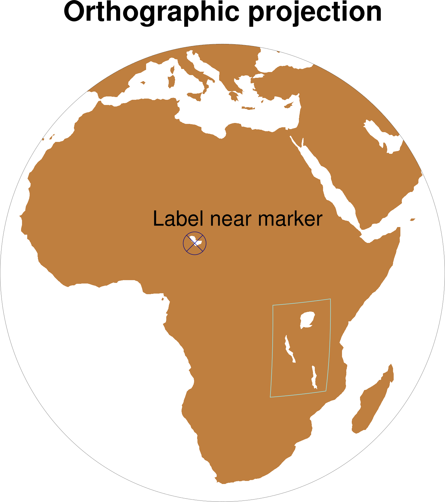
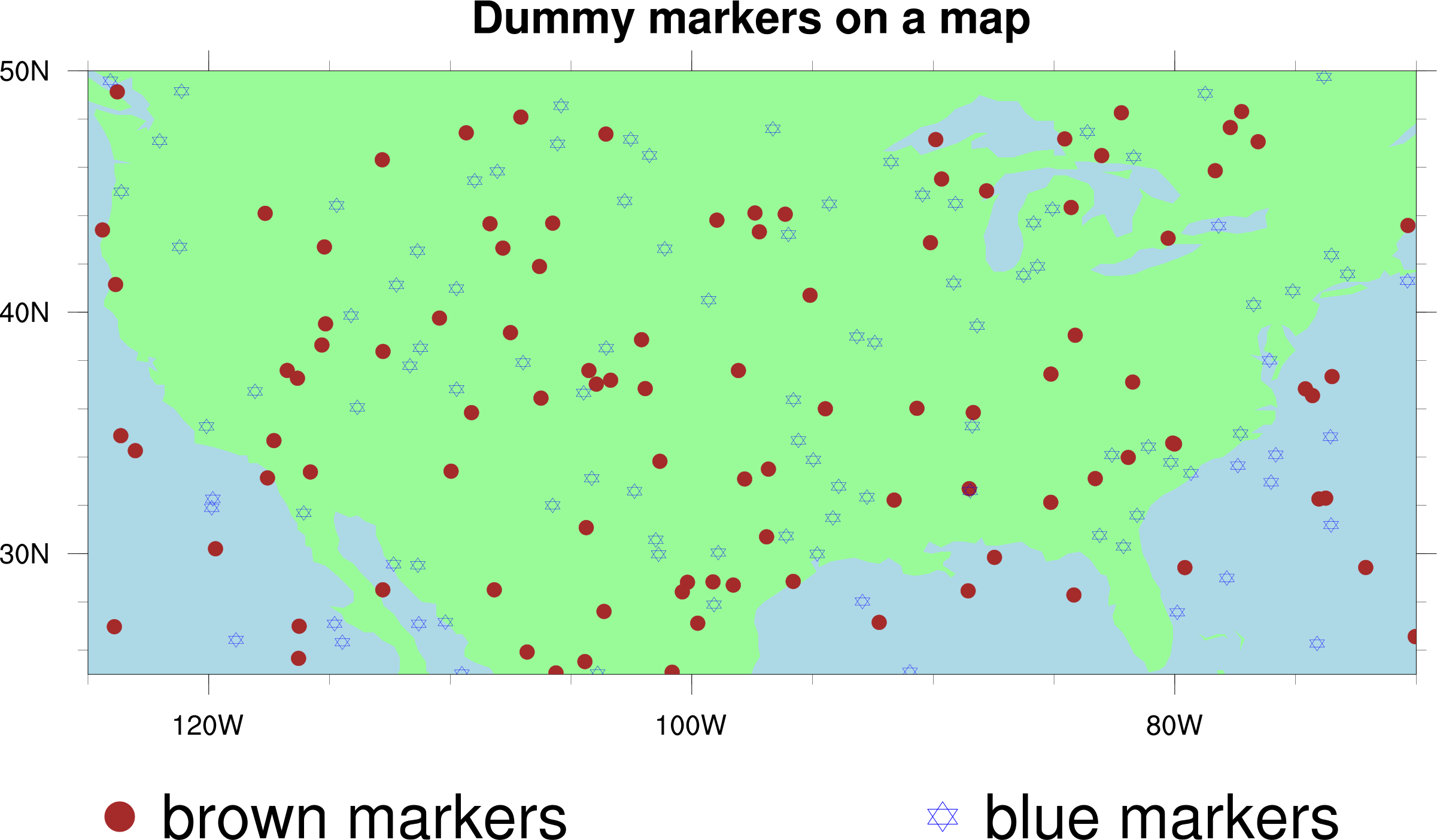
primitives


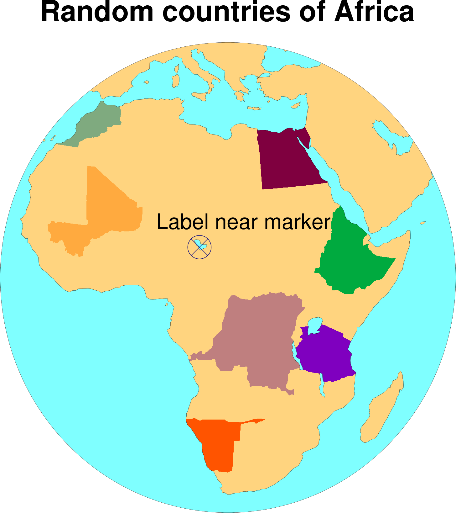
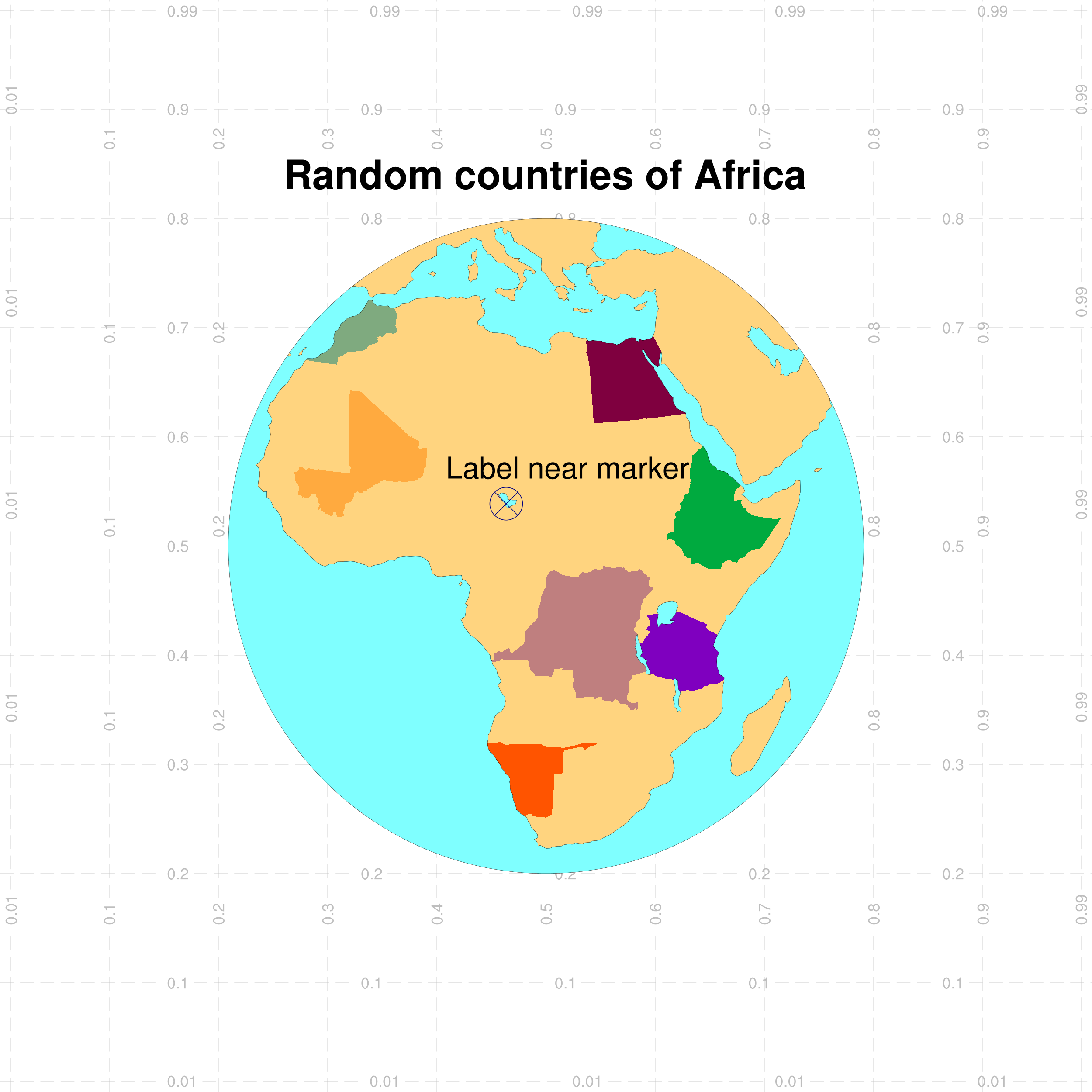
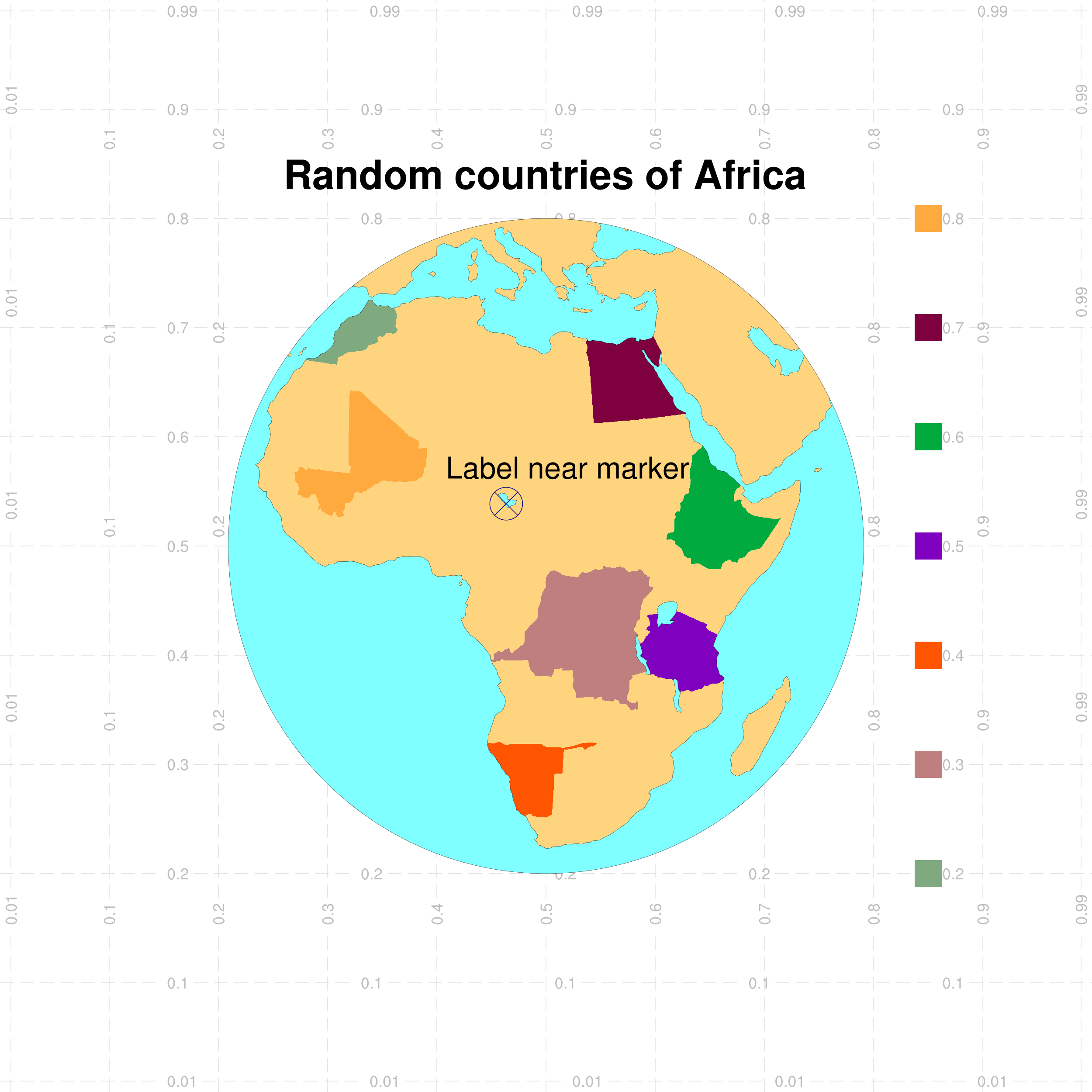
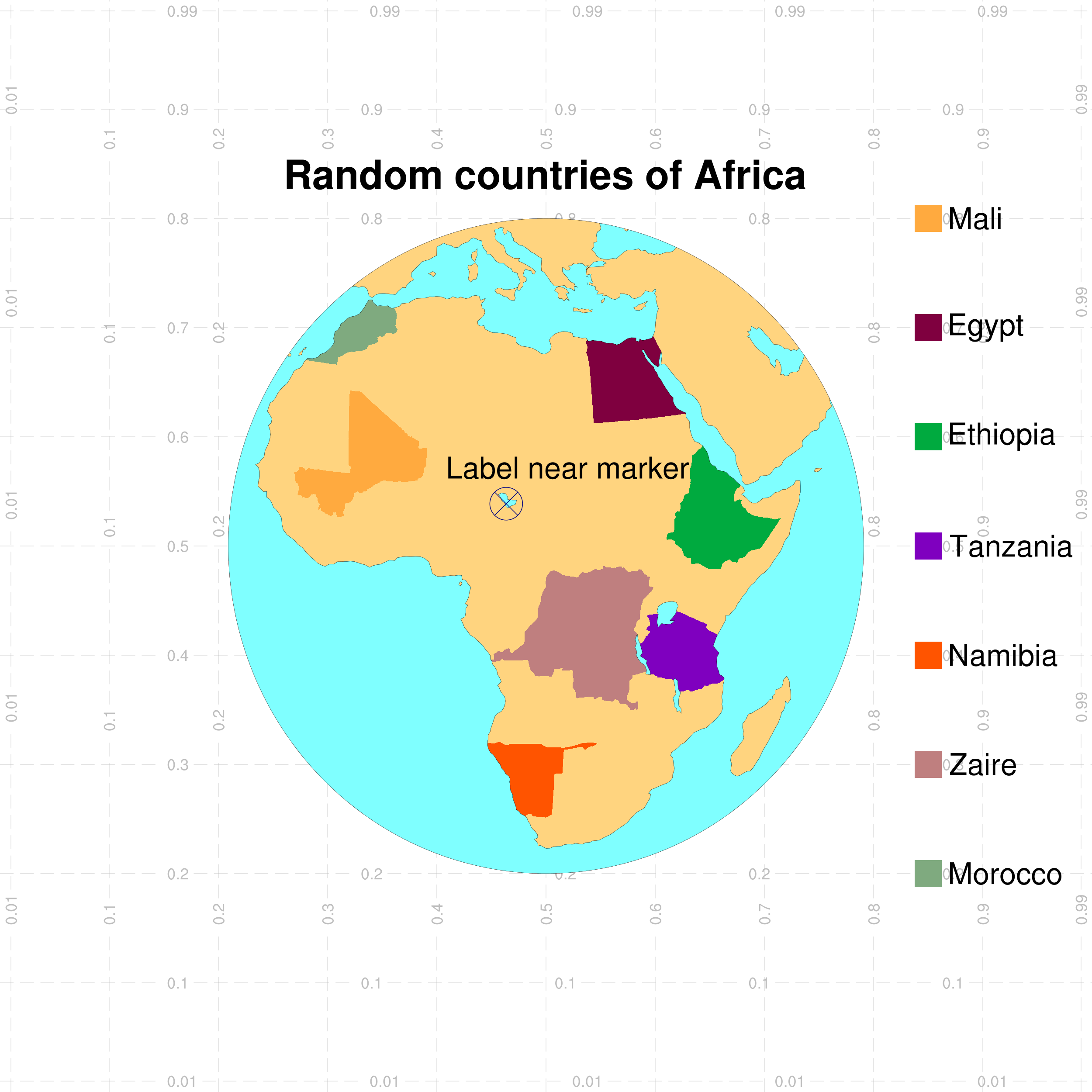
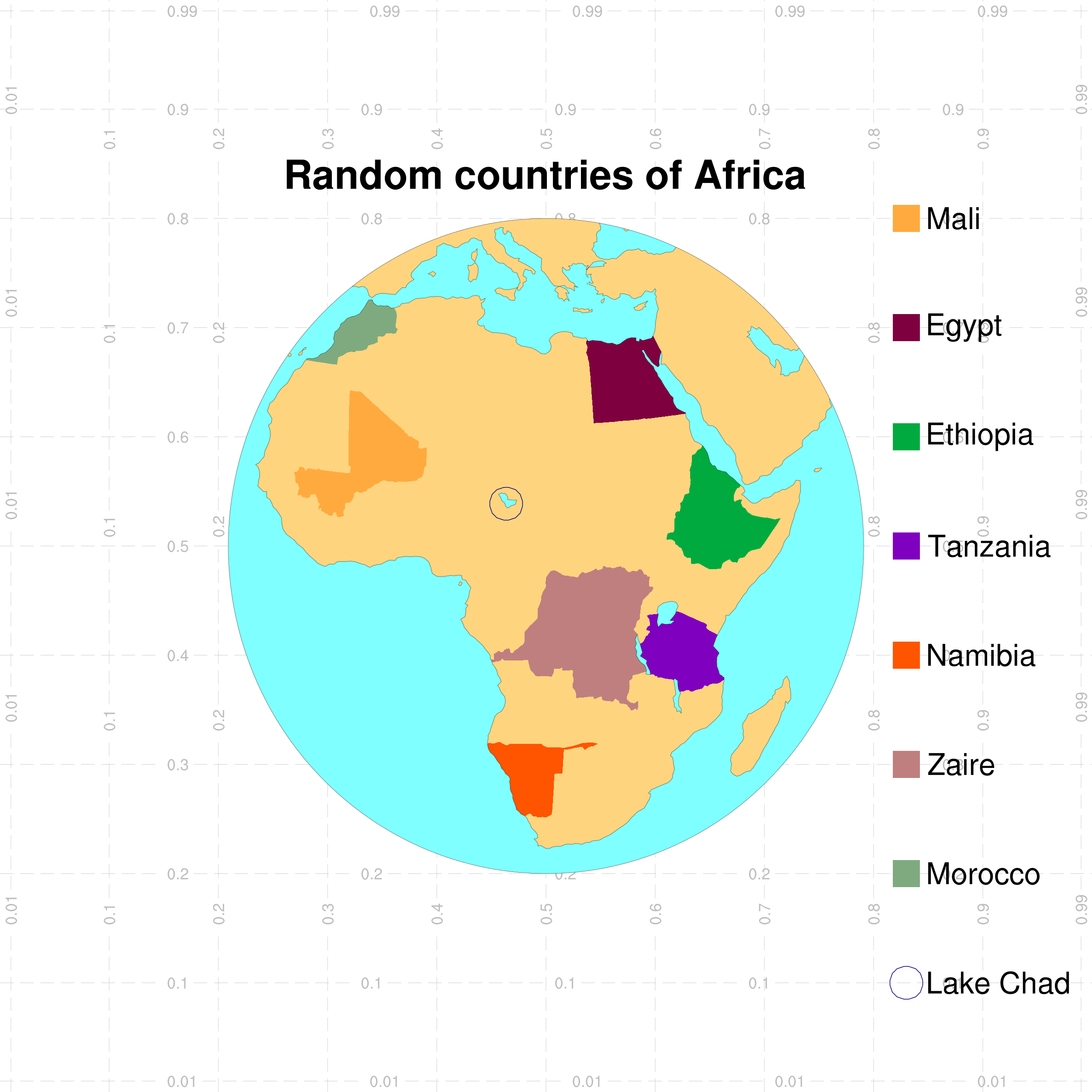
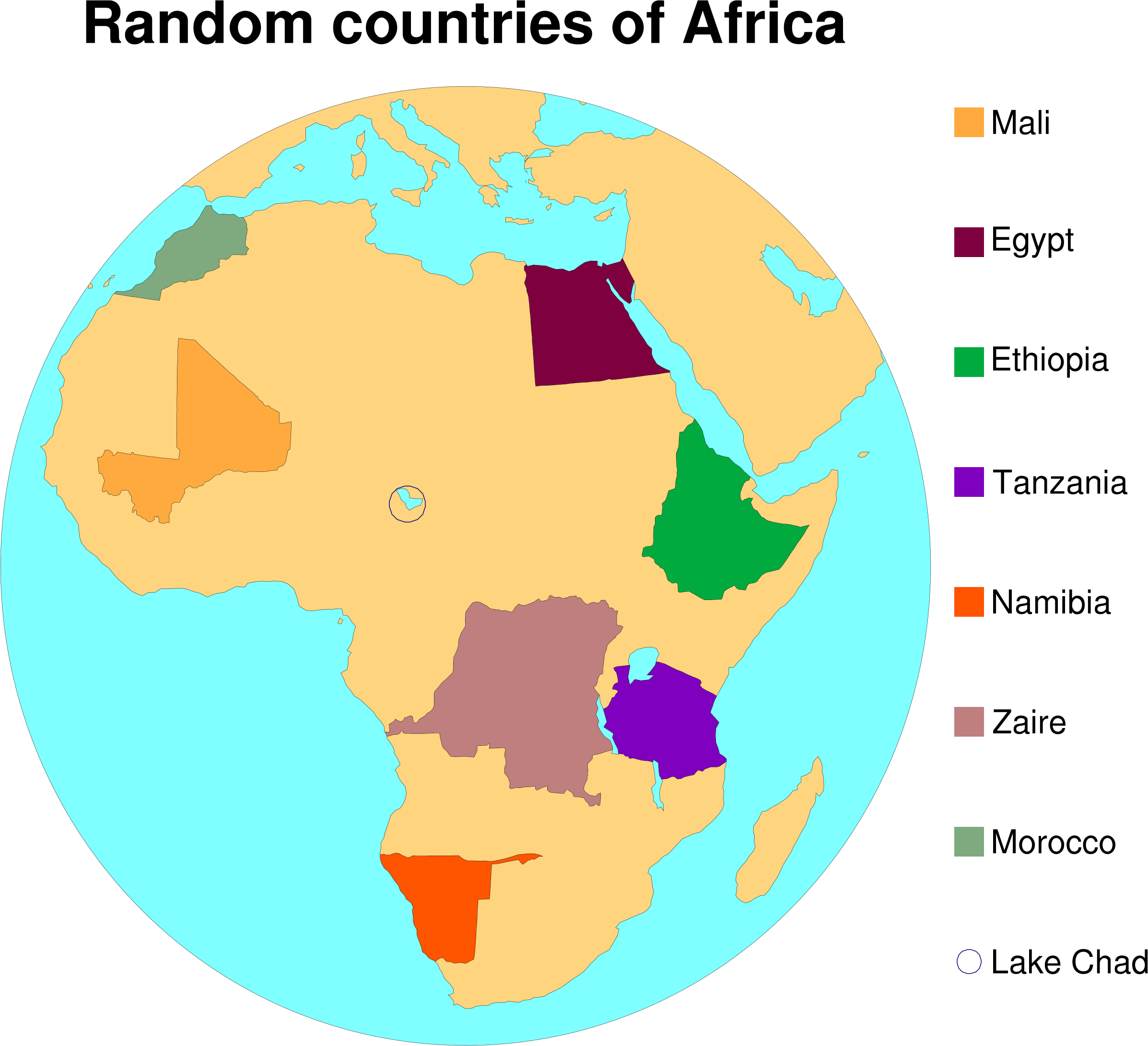
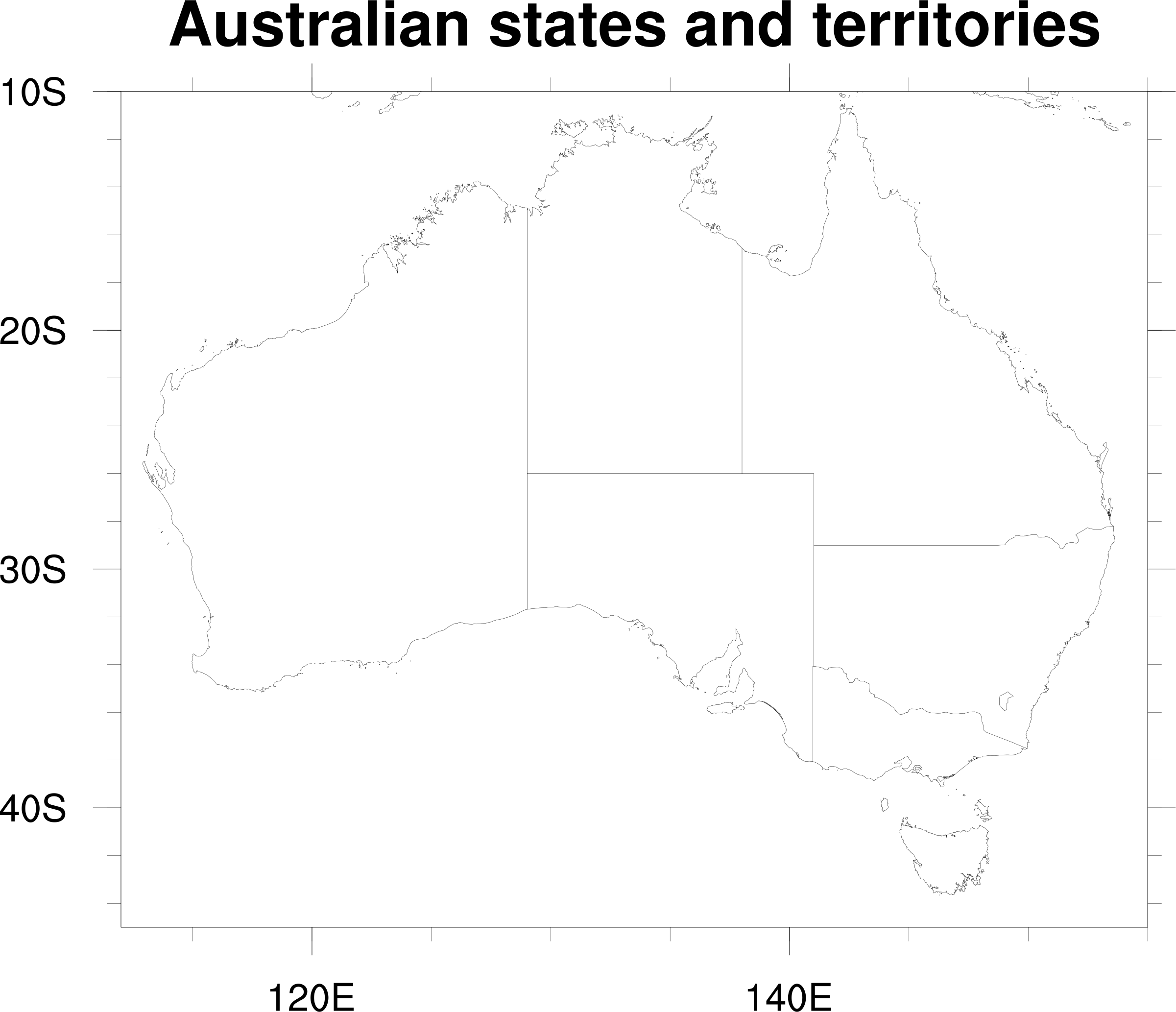

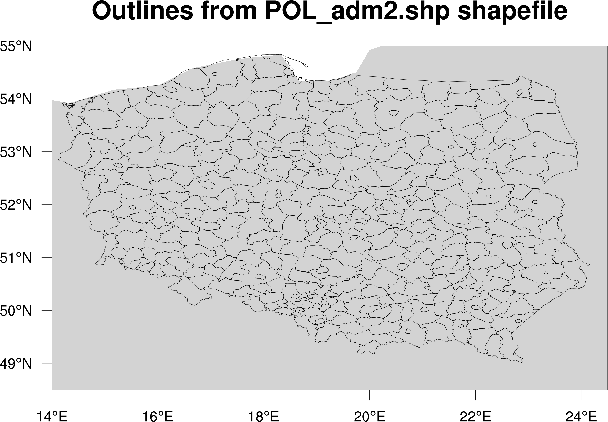
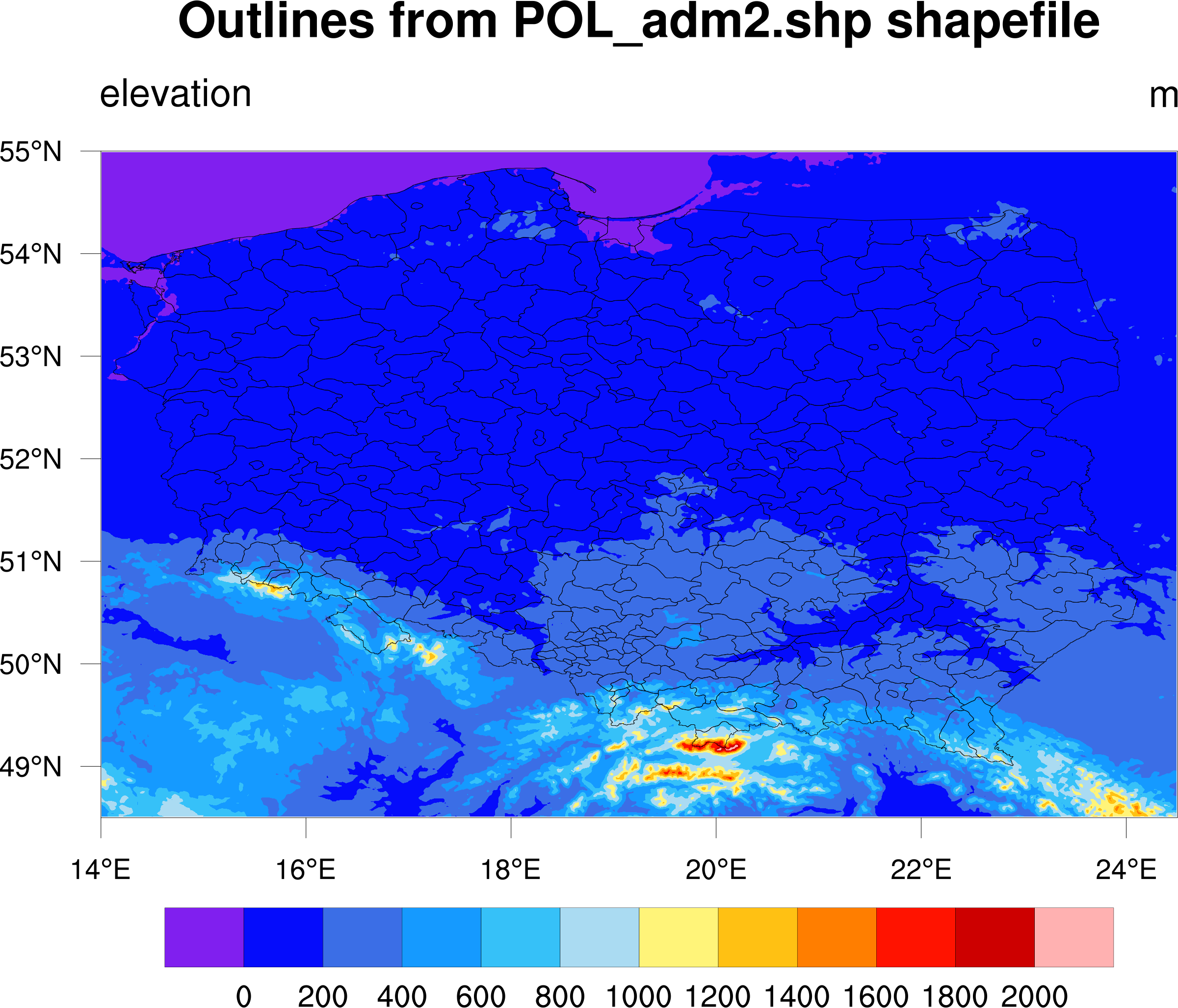
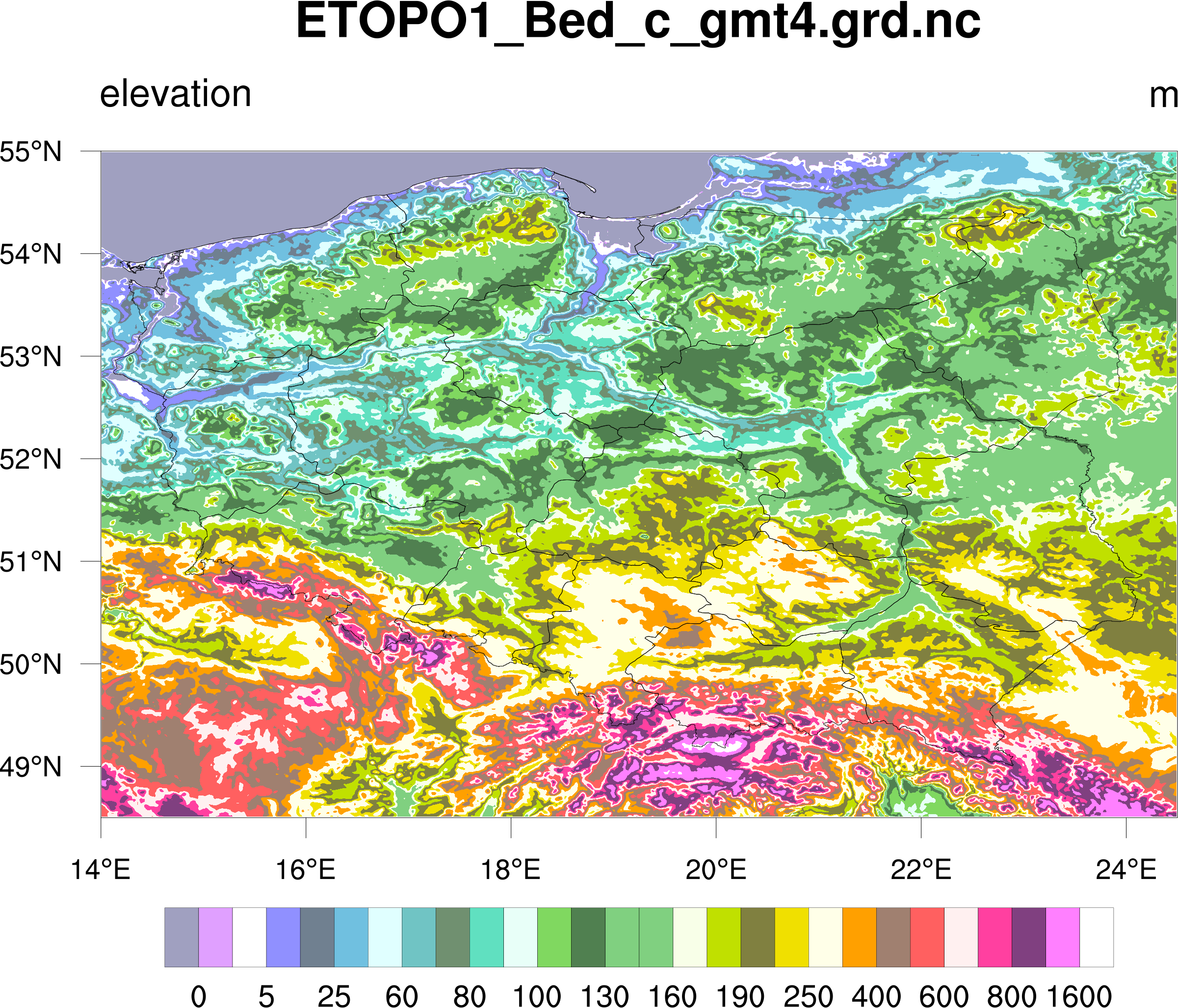
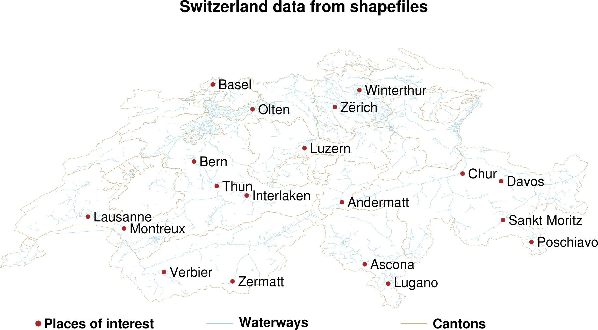
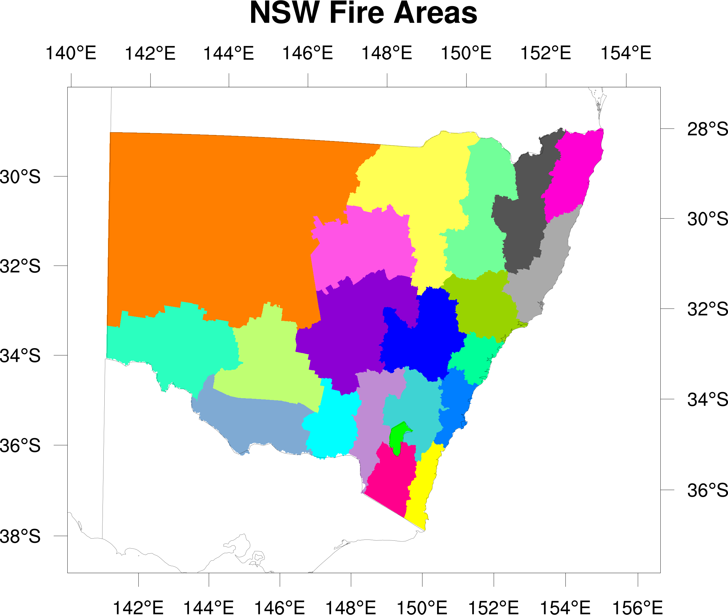
shapefile plots
| 
| 
| 
|
| shapefile1a.ncl | shapefile1b.ncl | shapefile1c.ncl | shapefile1d.ncl |
|
|
| 
| 
|
| colorado_map.ncl | france_shapefiles.ncl | switzerland_shapefiles.ncl | poly3h.ncl |
| 
| ||
| wrfgsn_hgt_shapefiles.ncl | wrfgsn_hgt_shapefiles_zoom.ncl |
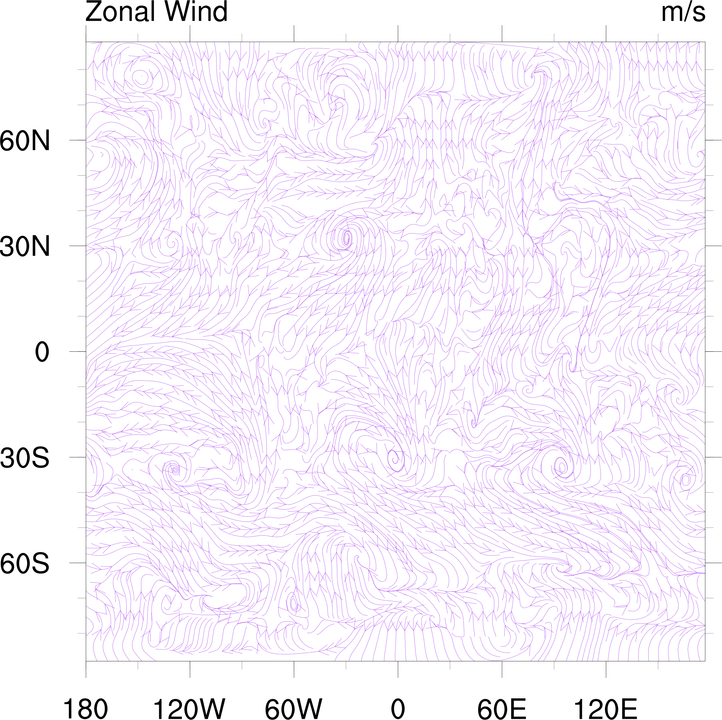
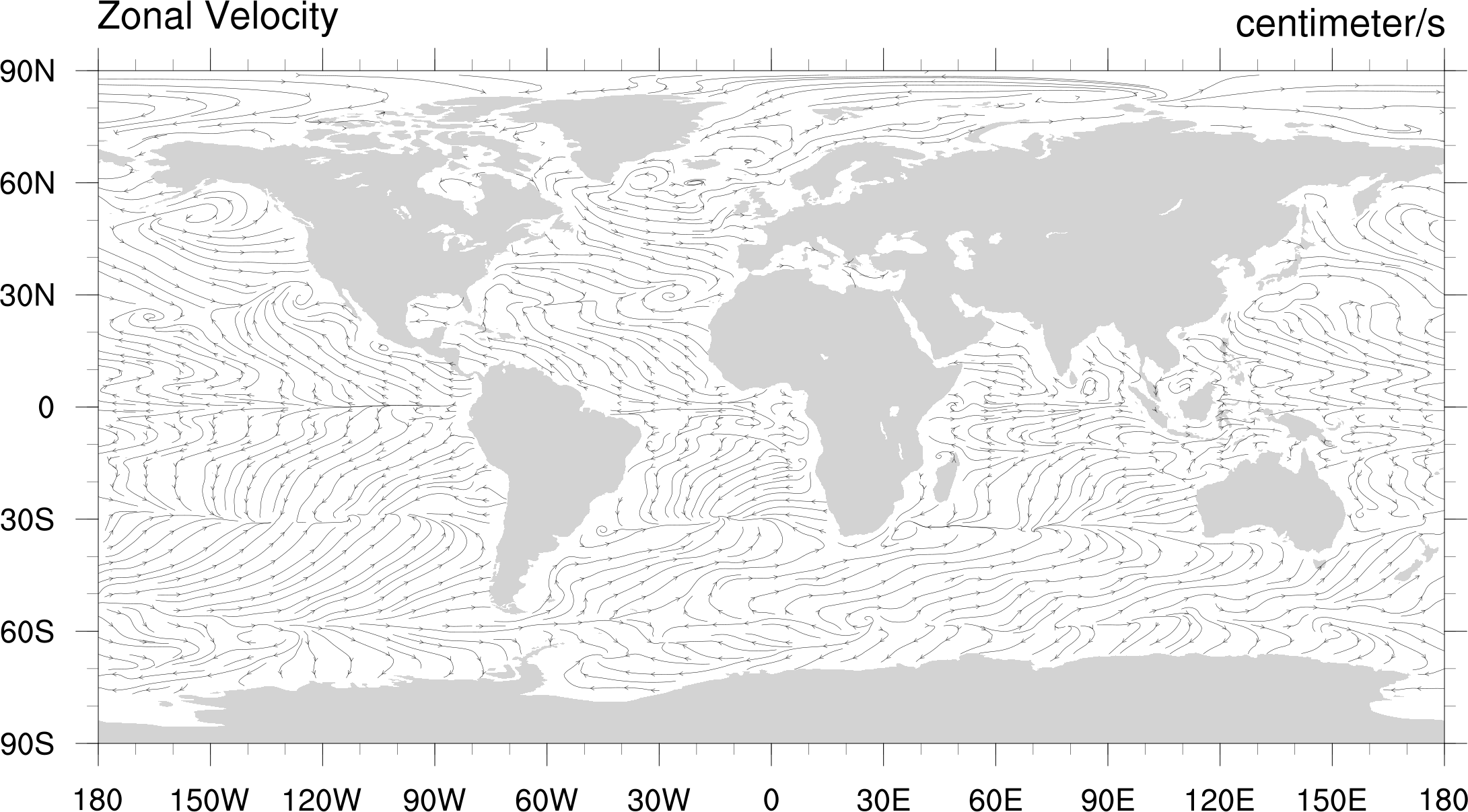
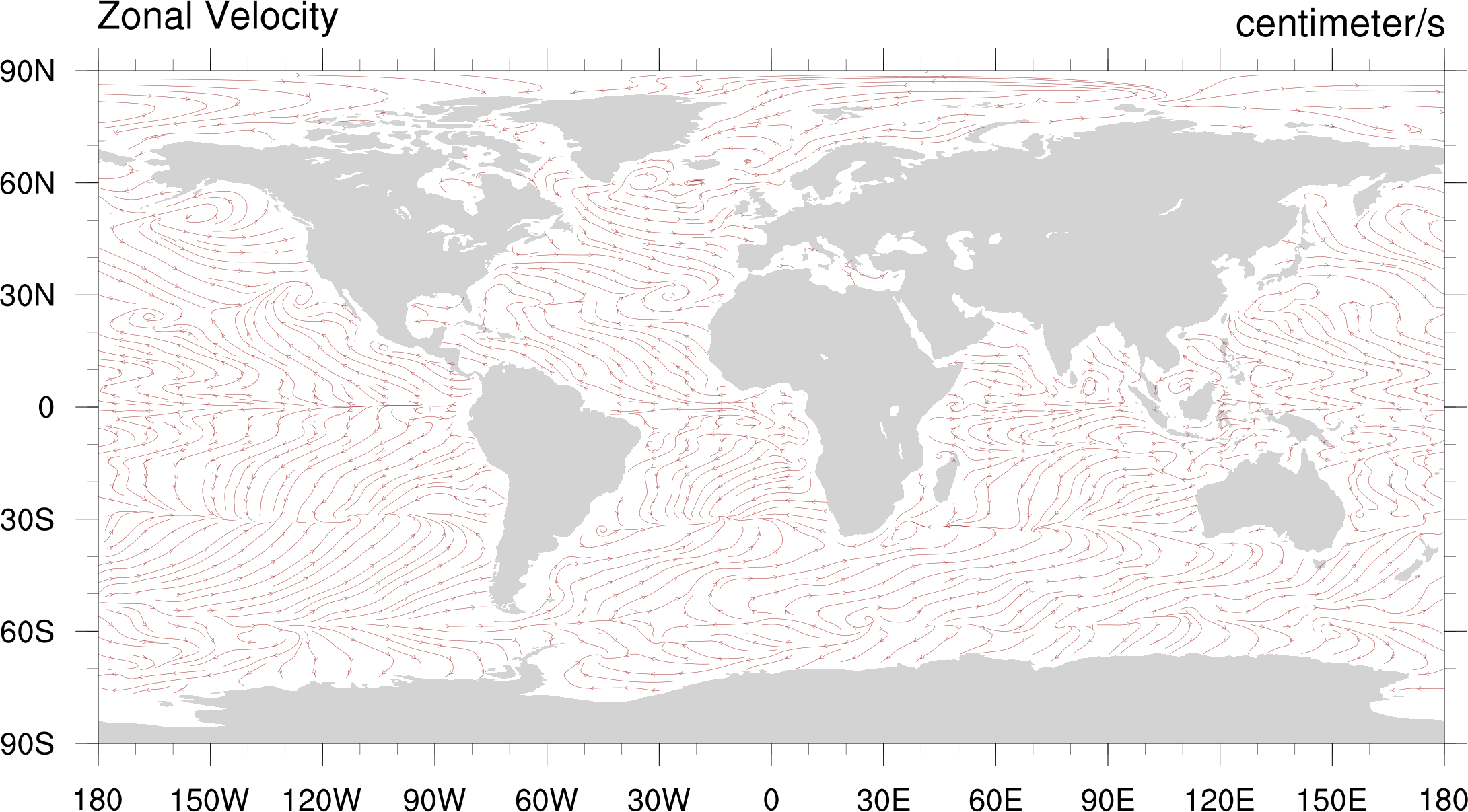
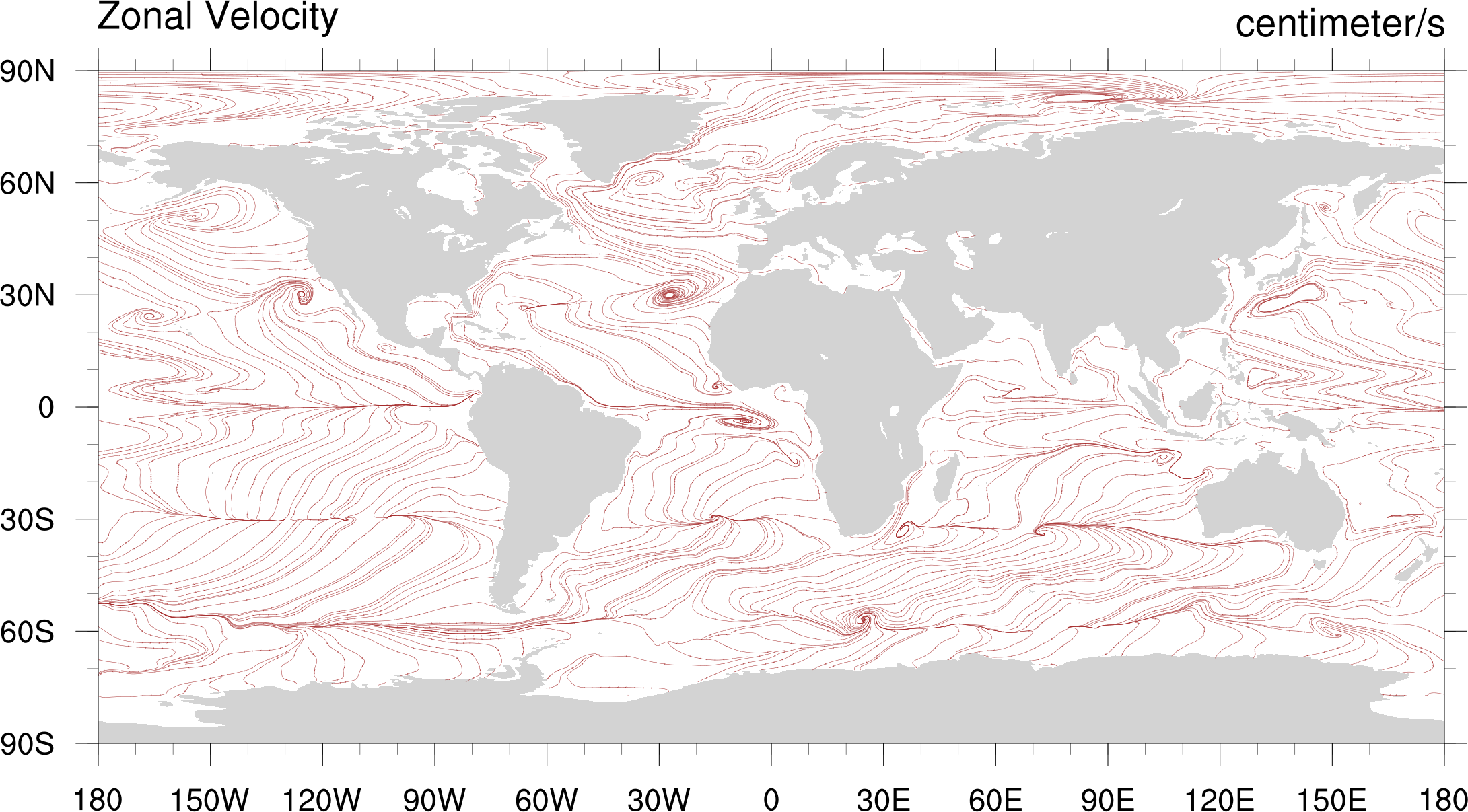
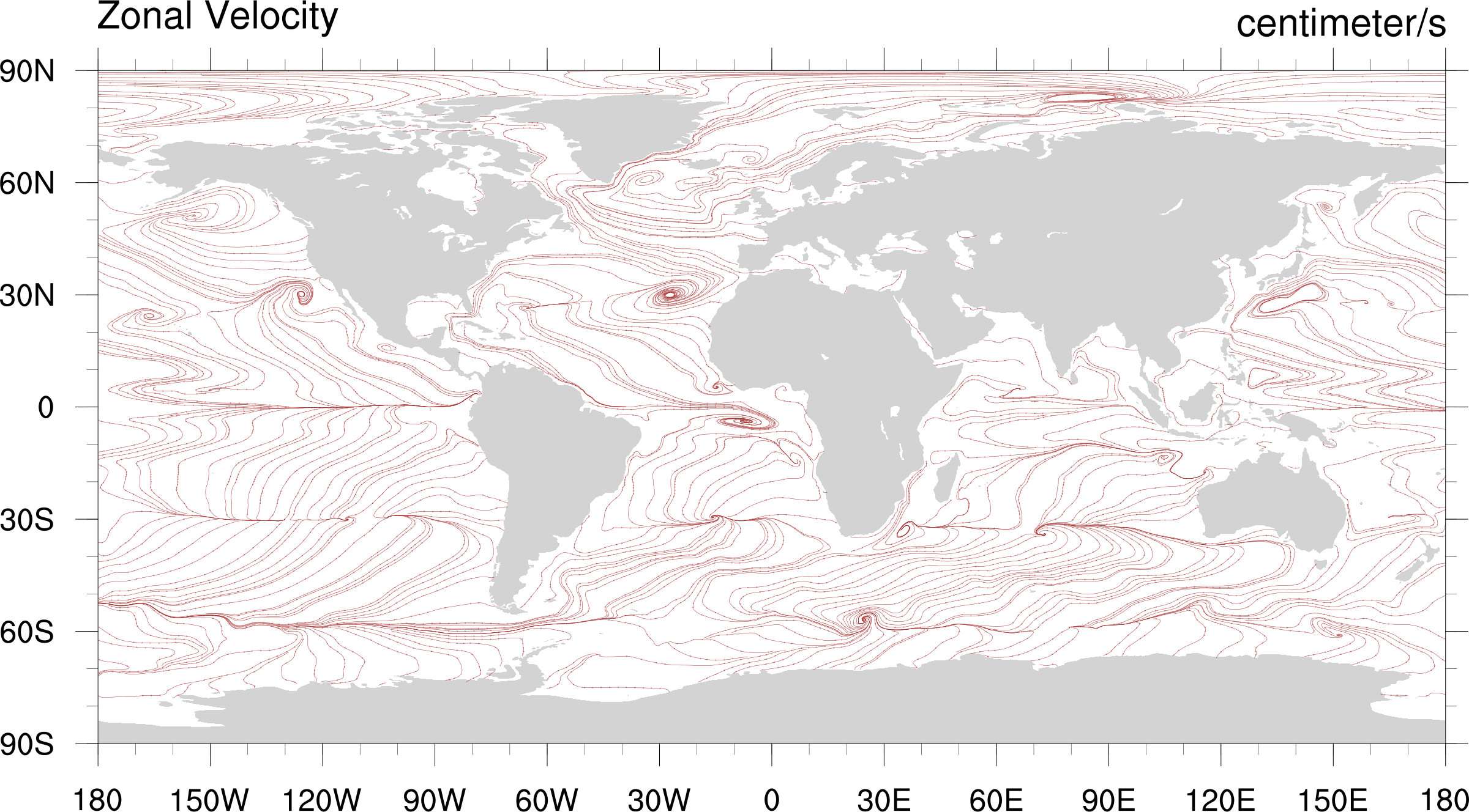
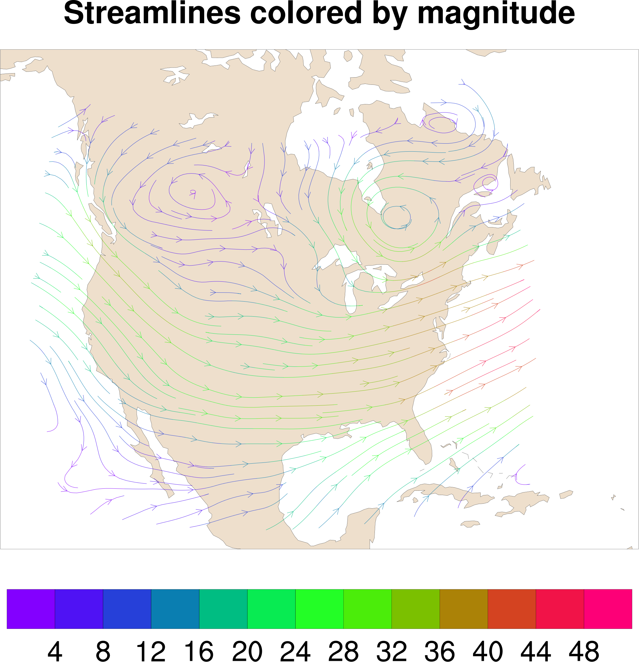
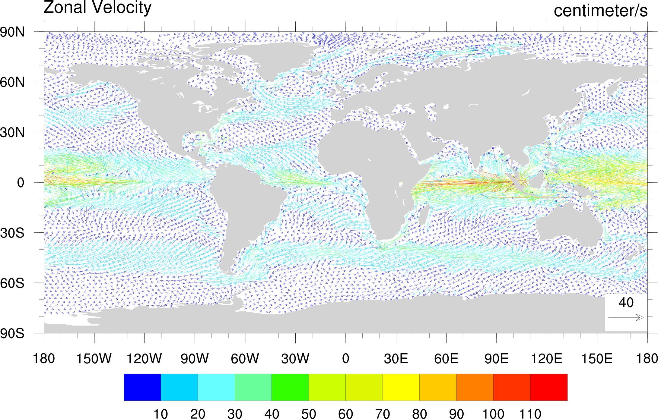
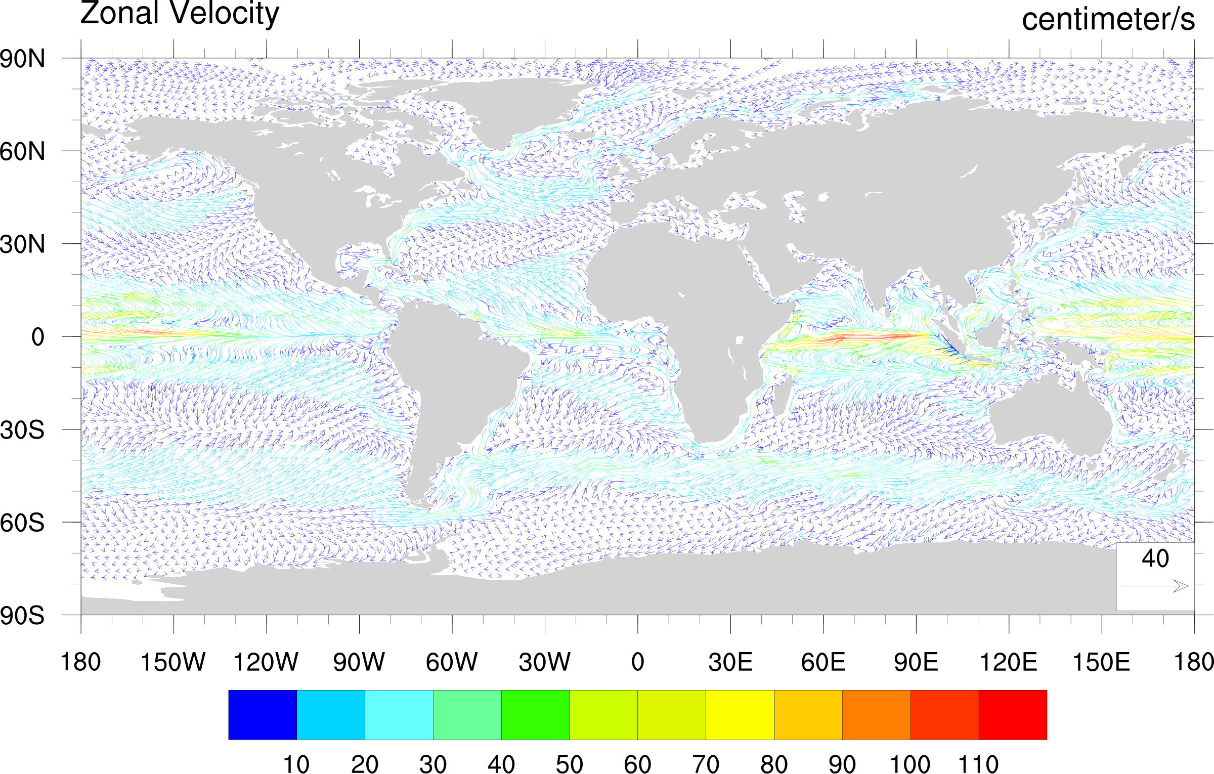
streamlines over maps
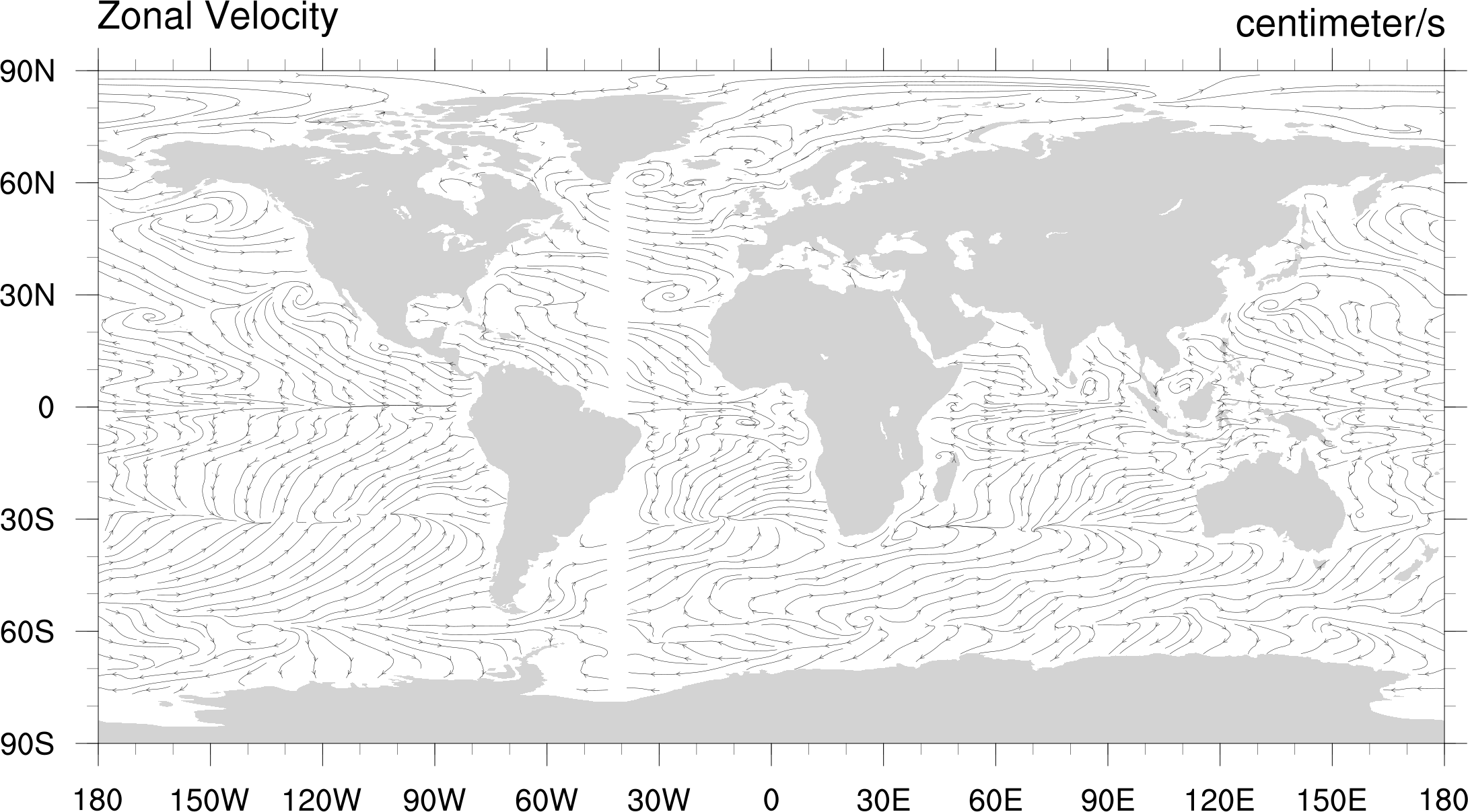
| 
| 
| 
|
| stream2a.ncl | stream2b.ncl | stream2c.ncl | stream2d.ncl |
| 
| 
| |
| stream2e.ncl | stream2f.ncl | streamline_map.ncl |
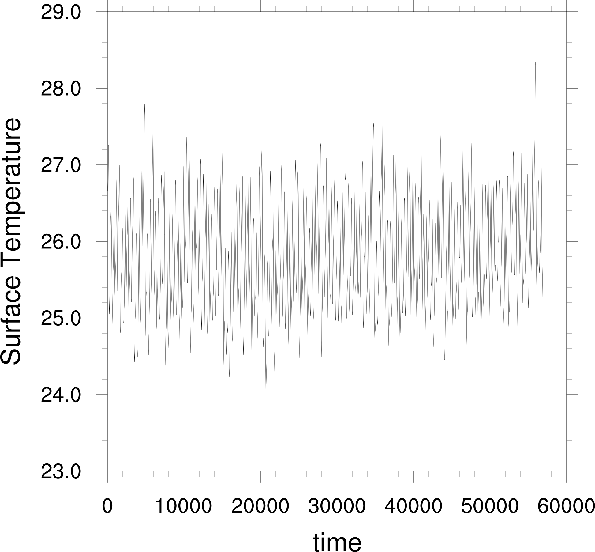
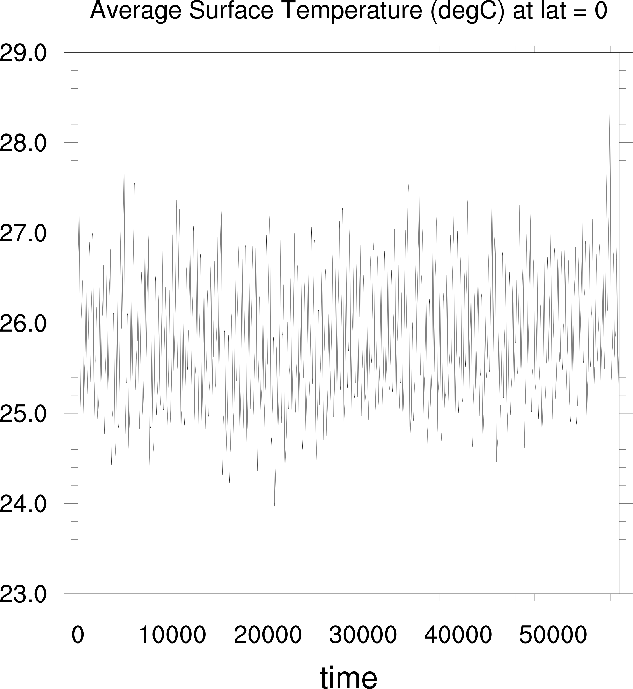
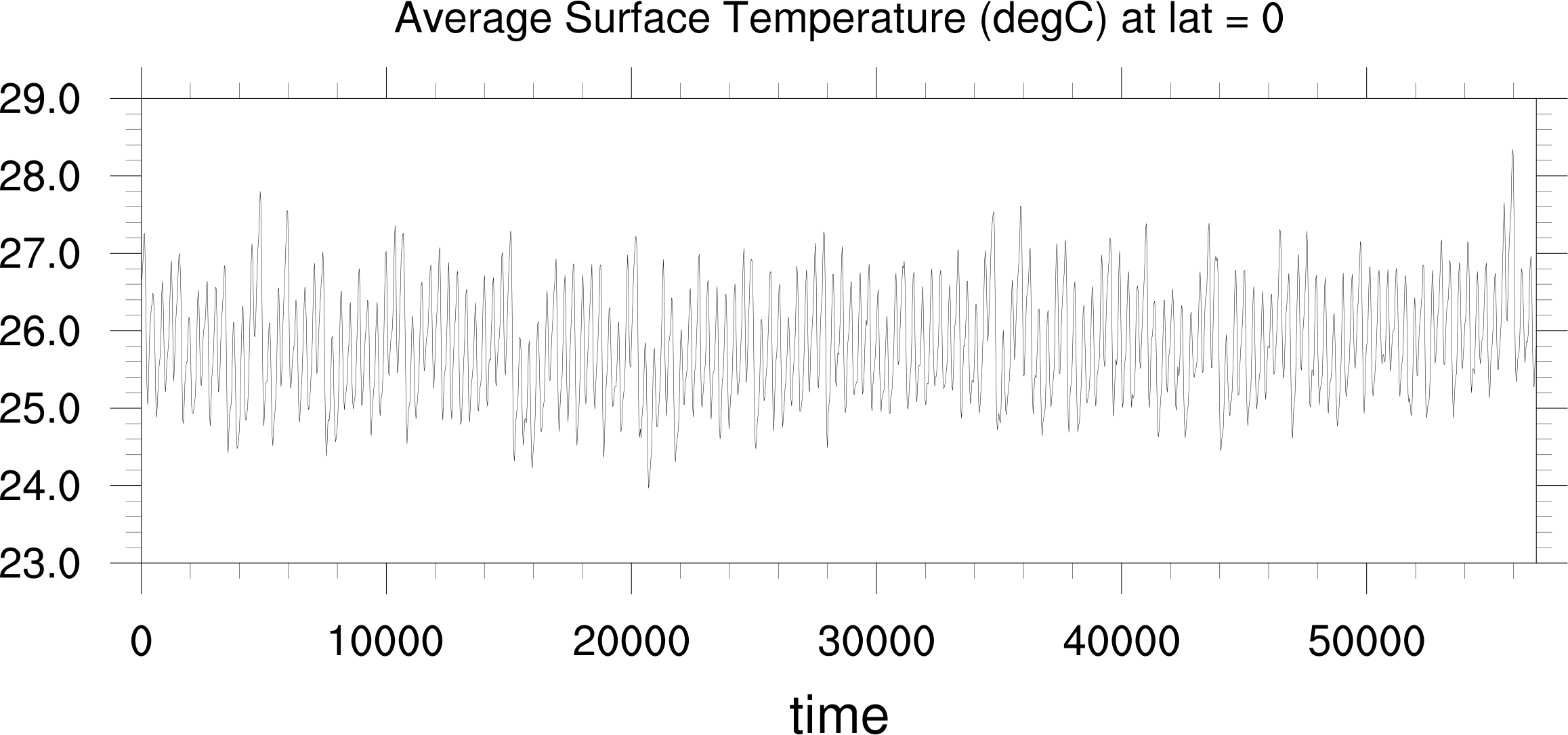
time series plots
| 
| 
| 
|
| time1a.ncl | time1b.ncl | time1c.ncl | time1d.ncl |
| 
| 
|
|
| time1e.ncl | time1f.ncl | time1g.ncl | time1h.ncl |
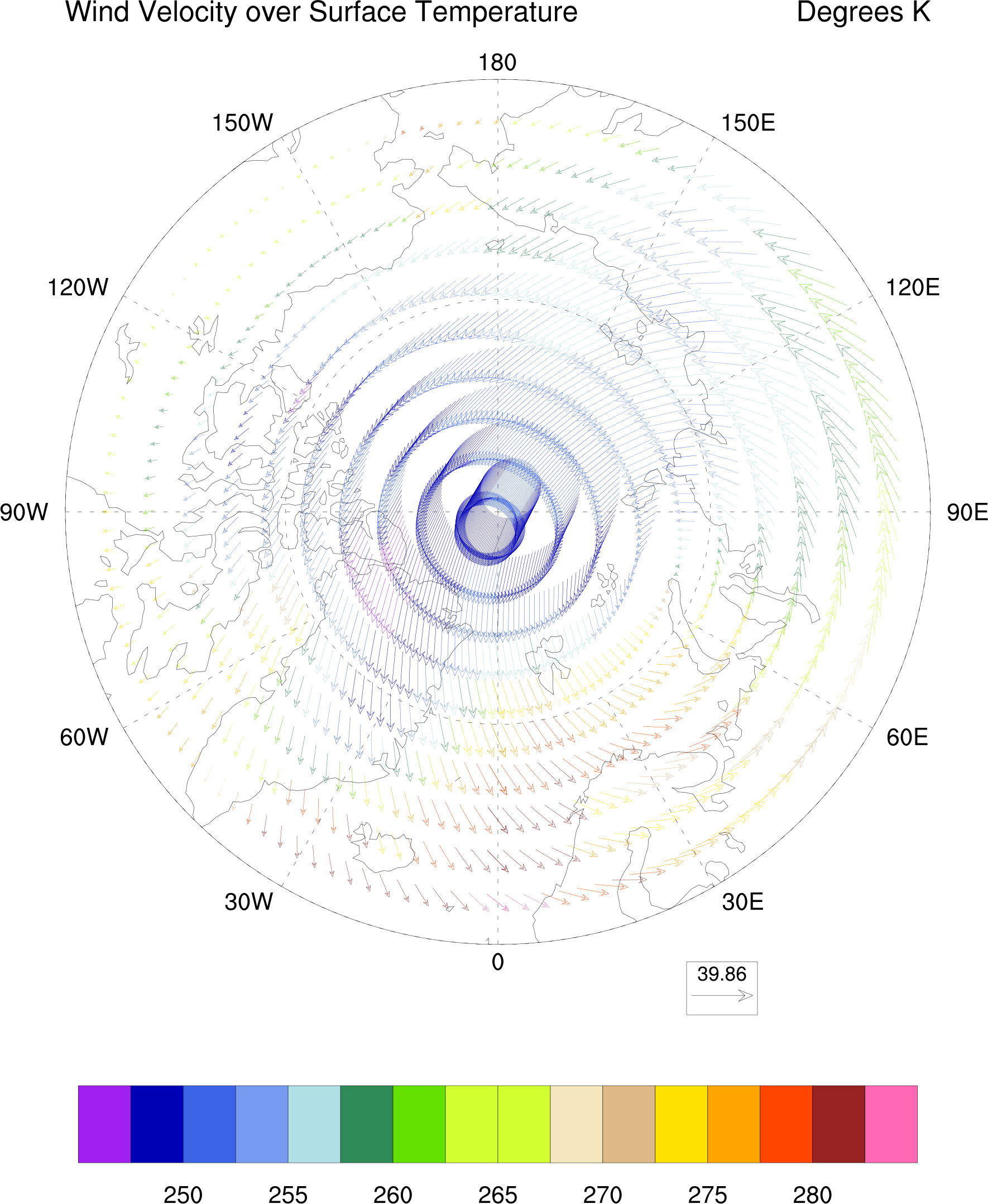
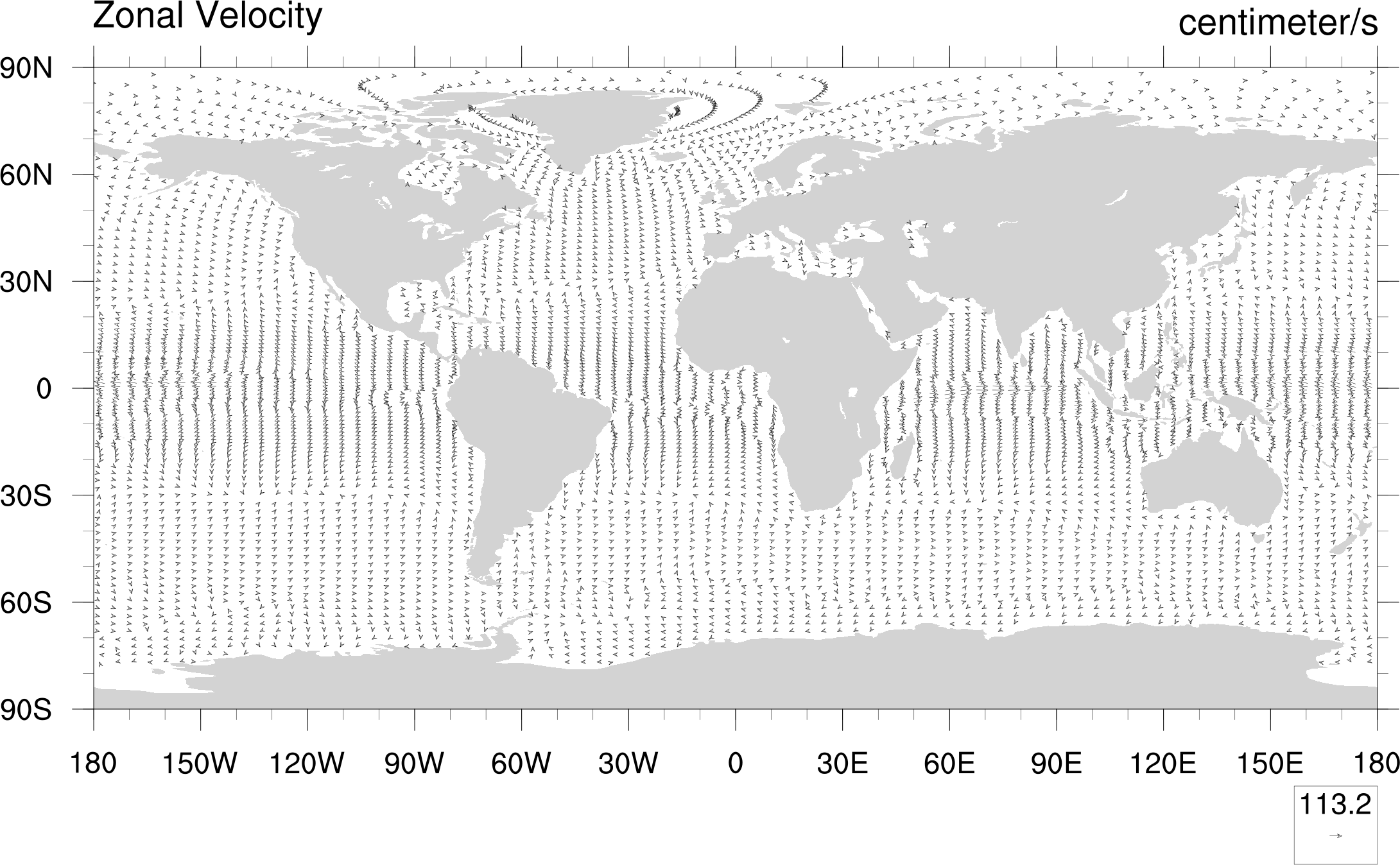
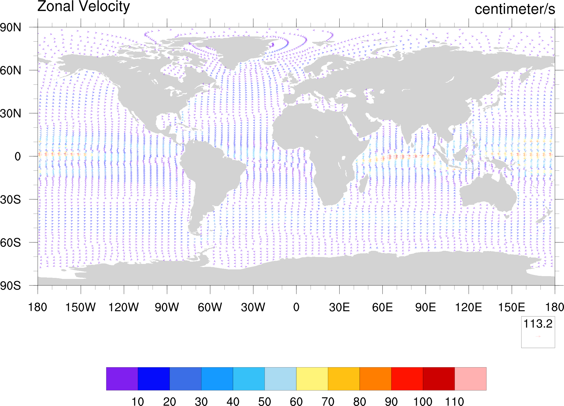
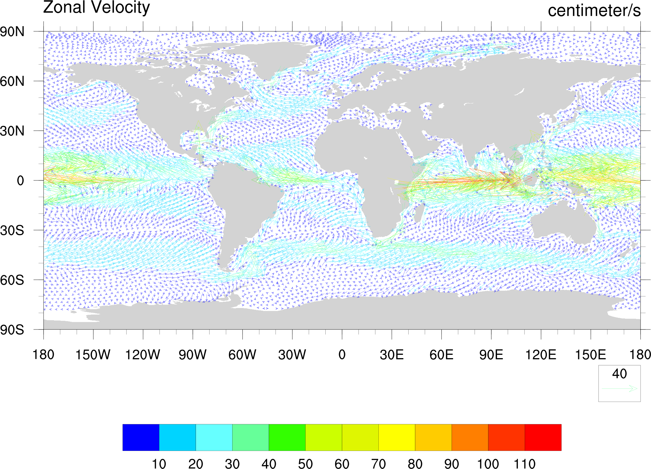
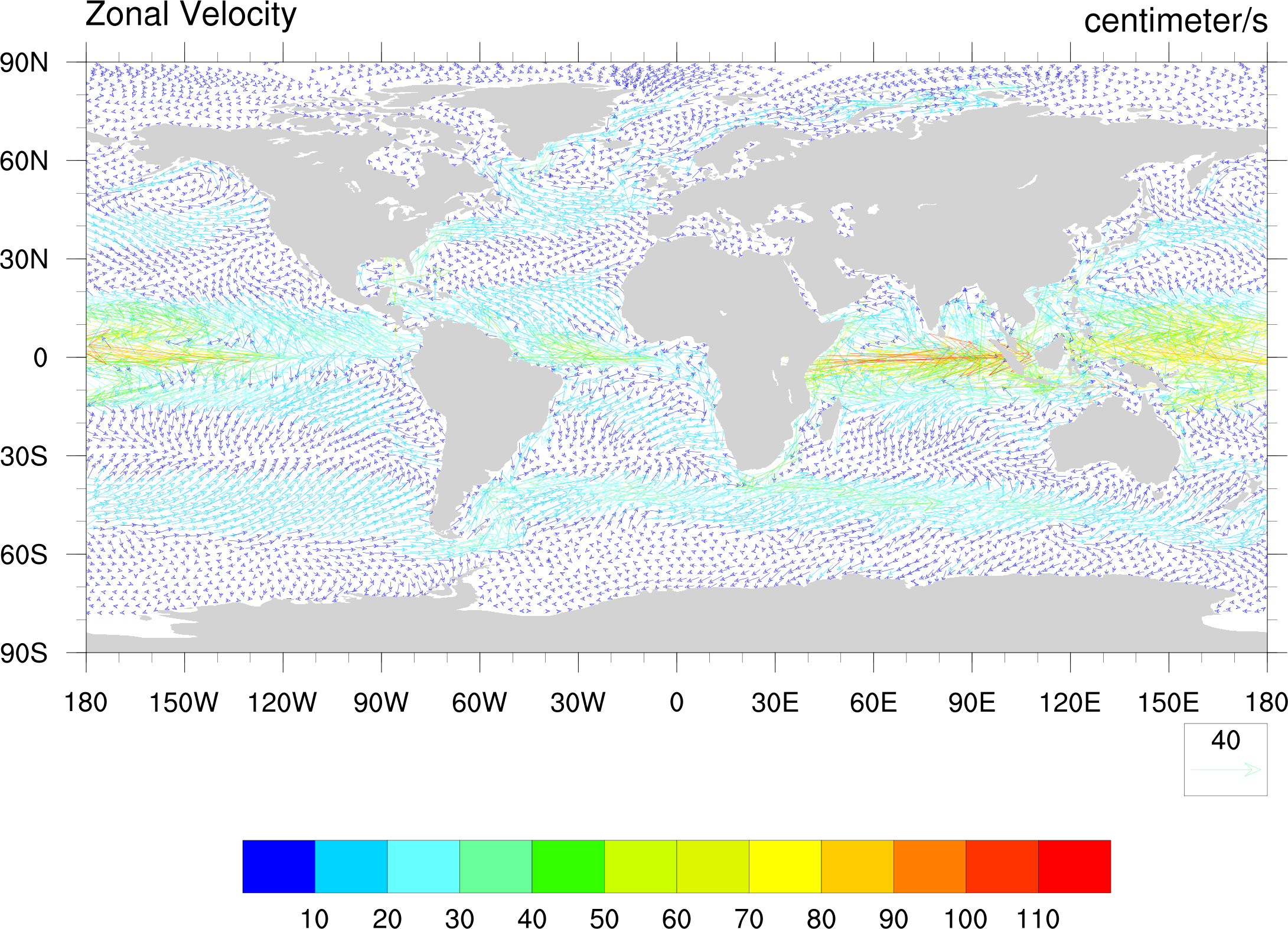
vectors over cylindrical equidistant maps
| 
| 
| 
|
| vector1a.ncl | vector1b.ncl | vector1c.ncl | vector1d.ncl |
| 
| 
| |
| vector1e.ncl | vector1f.ncl | vector1g.ncl |
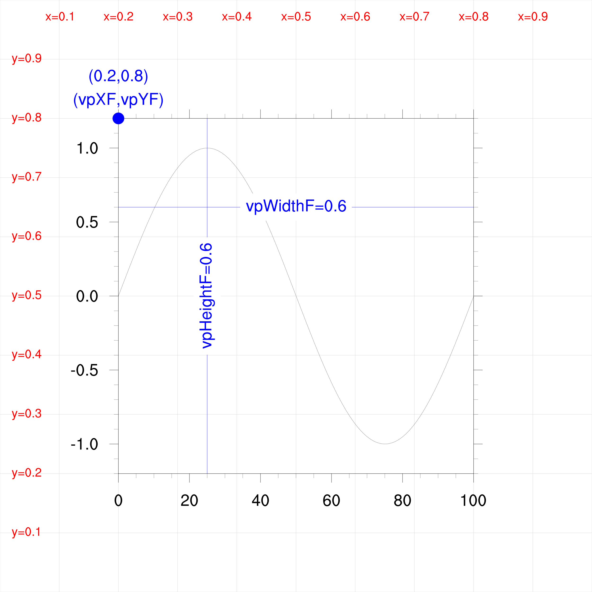
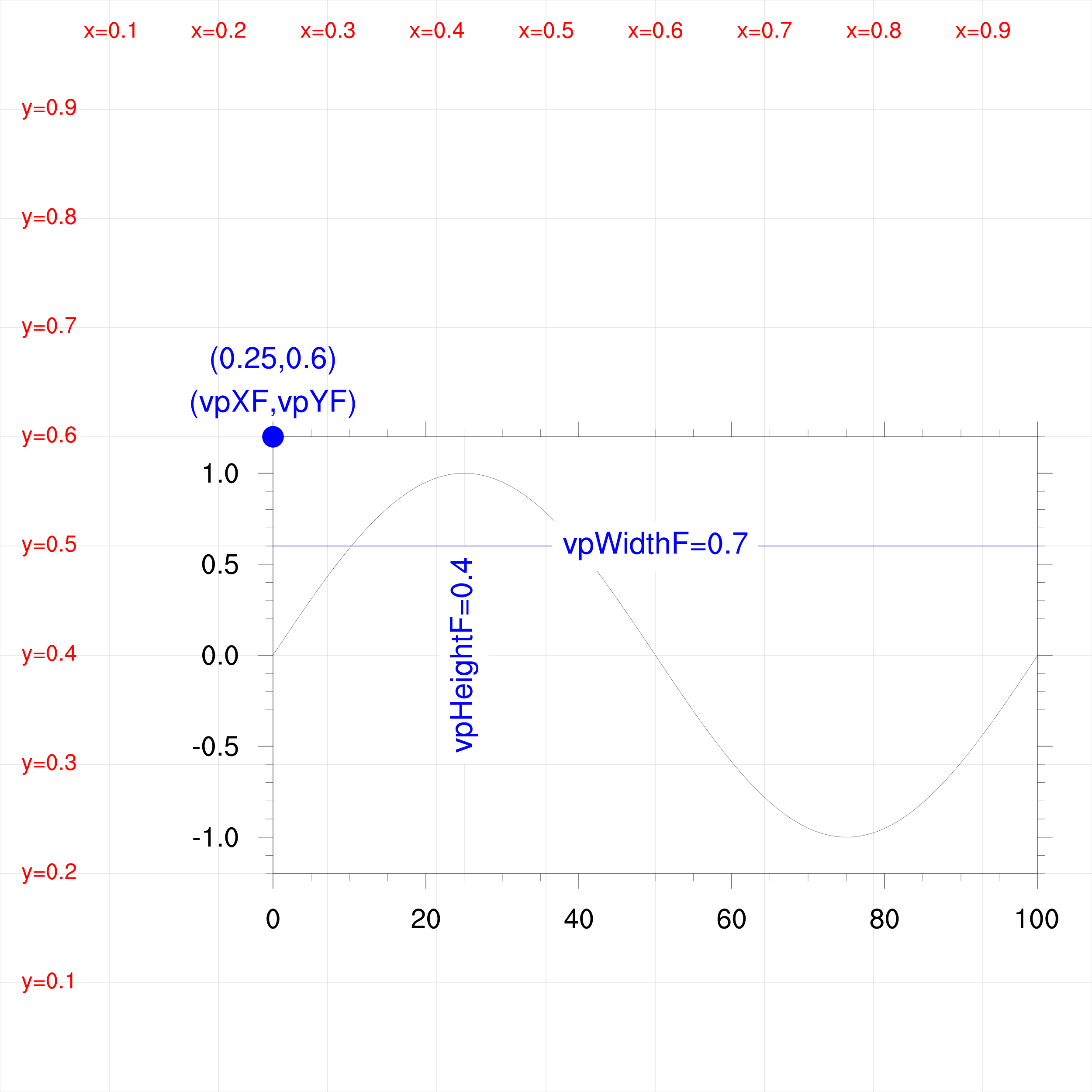
view port illustrations
| 
| 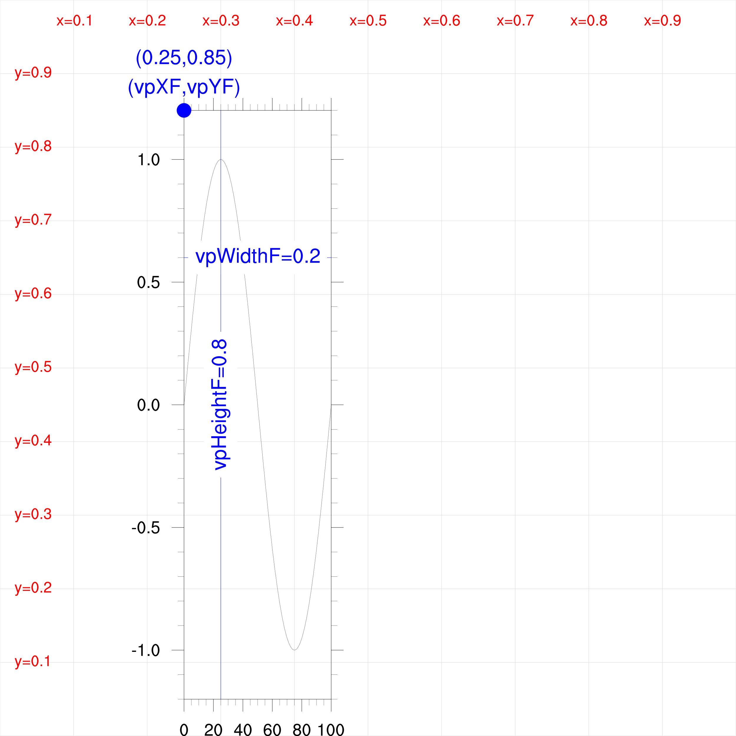
|
| vp1a.ncl
view.ncl | vp1b.ncl
view.ncl | vp1c.ncl
view.ncl |
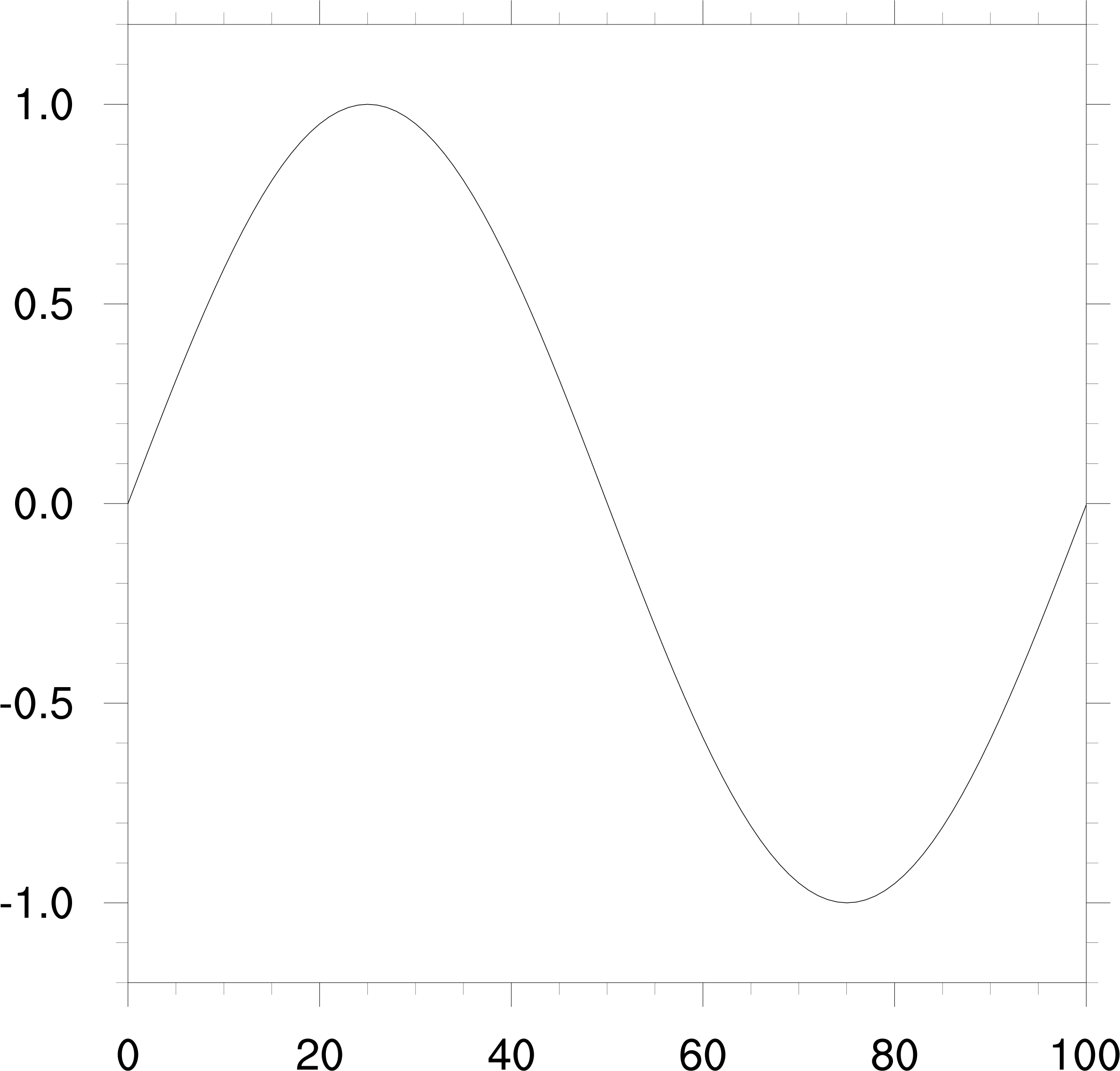
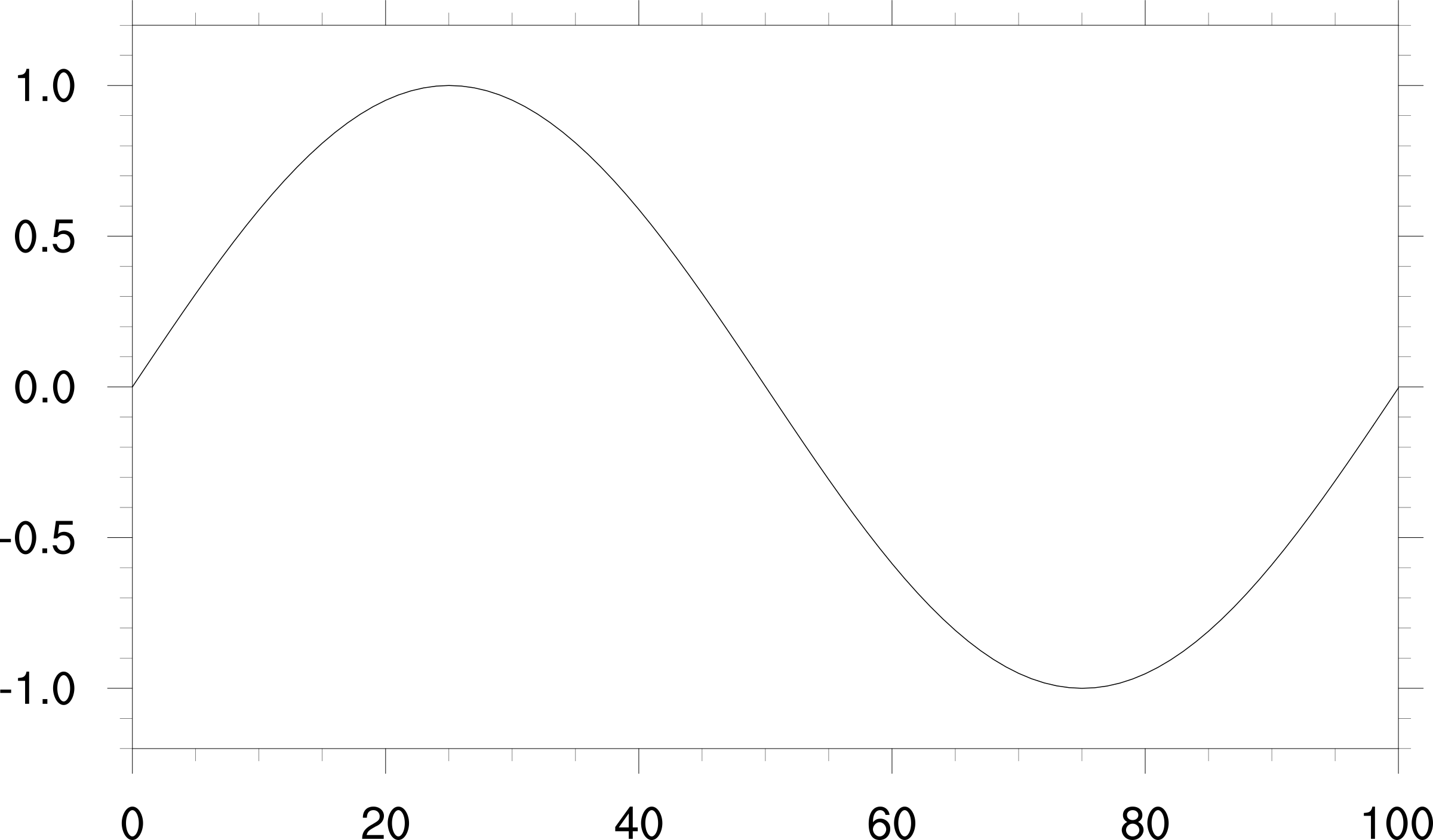
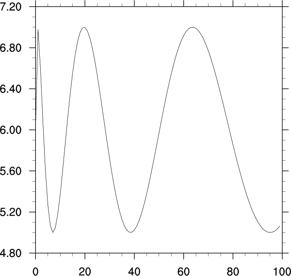
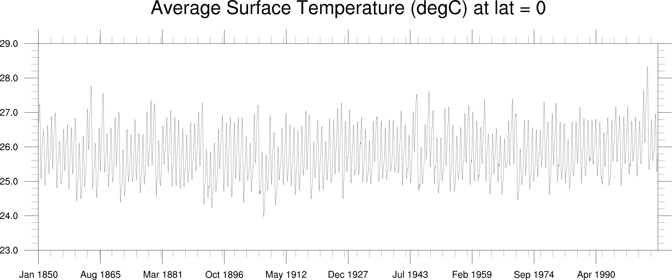
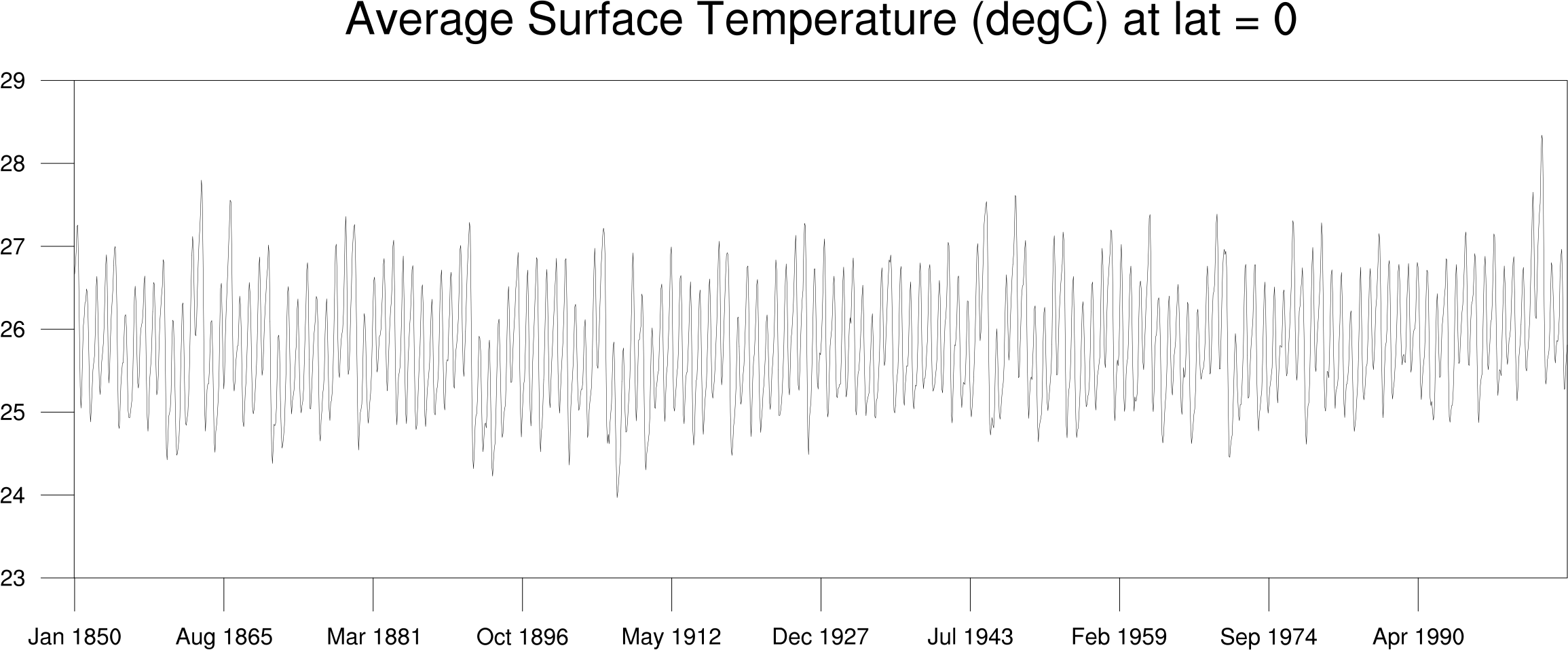
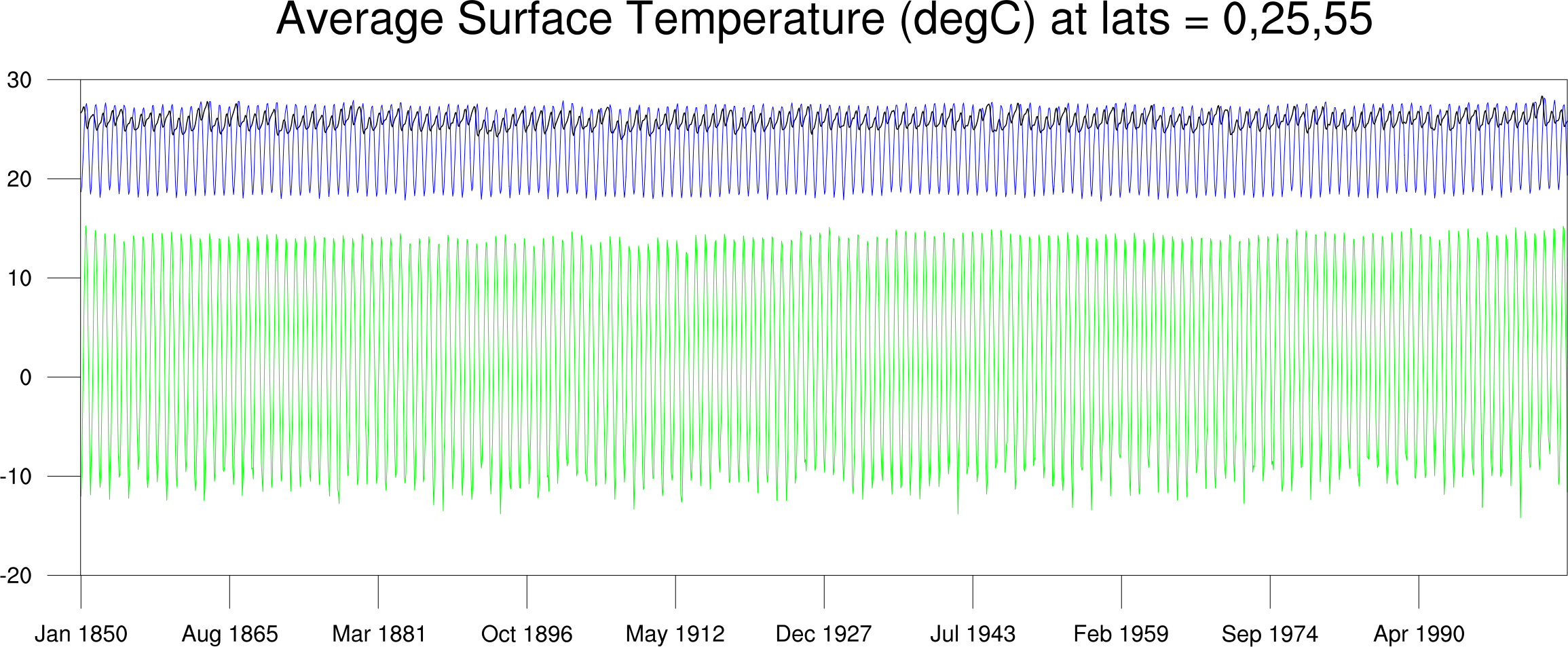
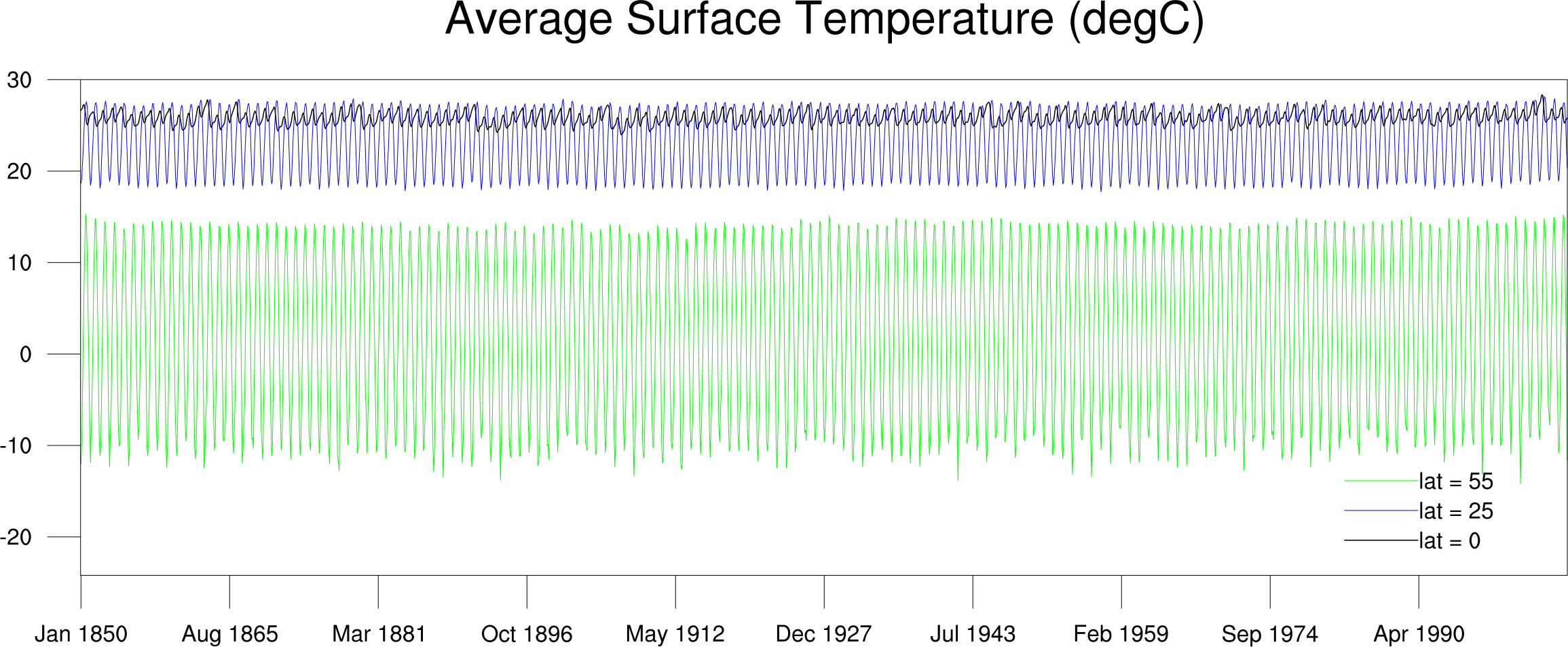
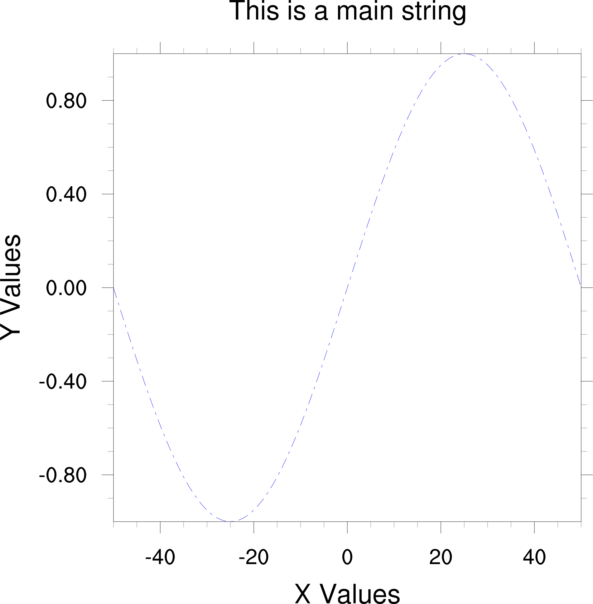
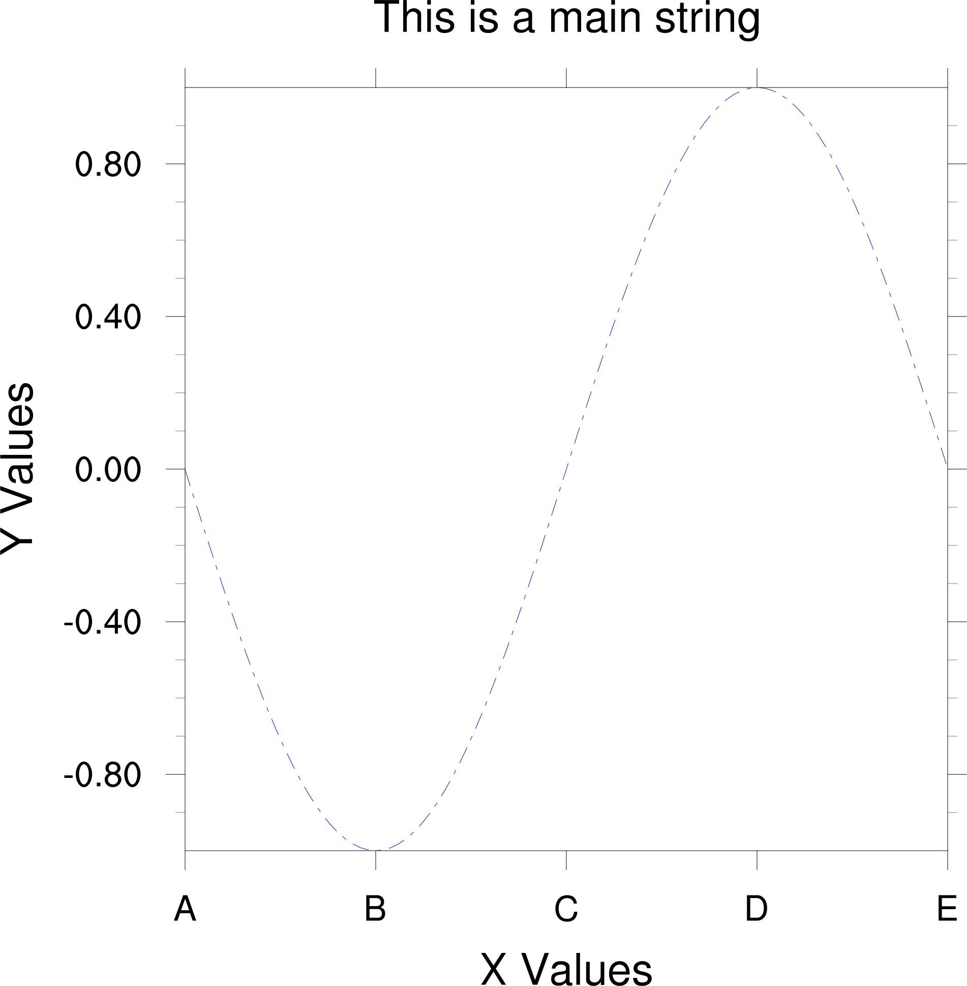
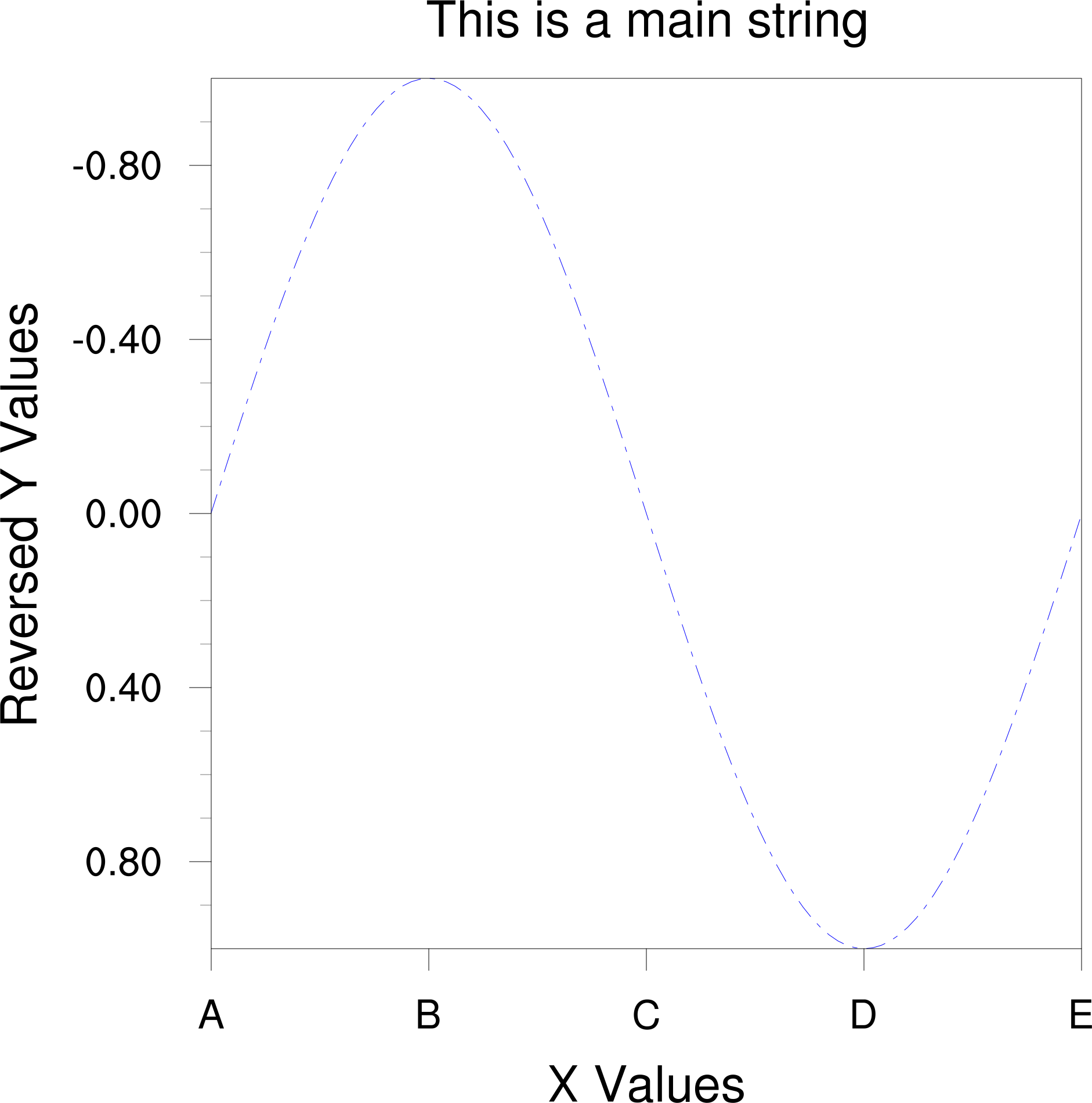
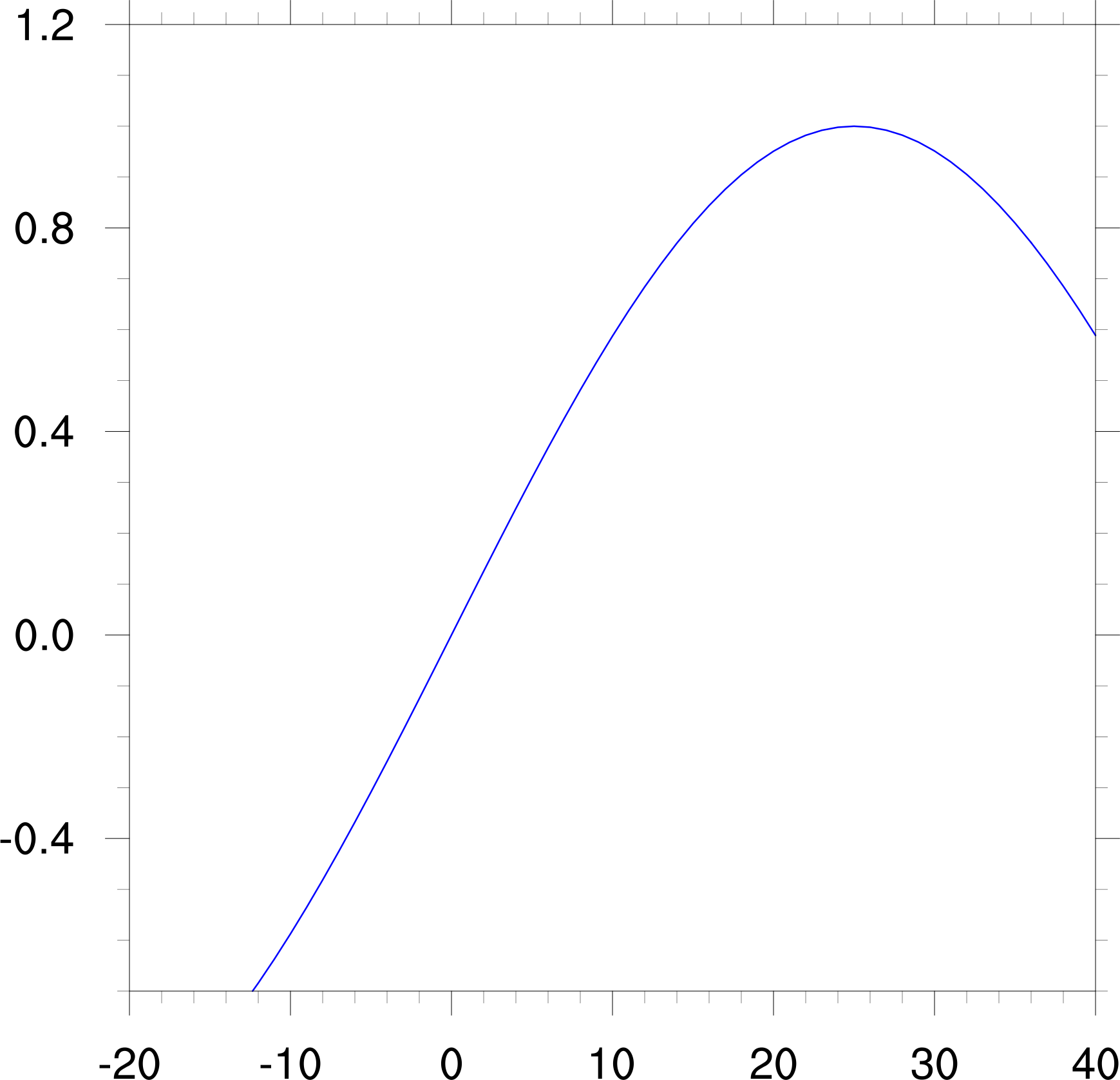
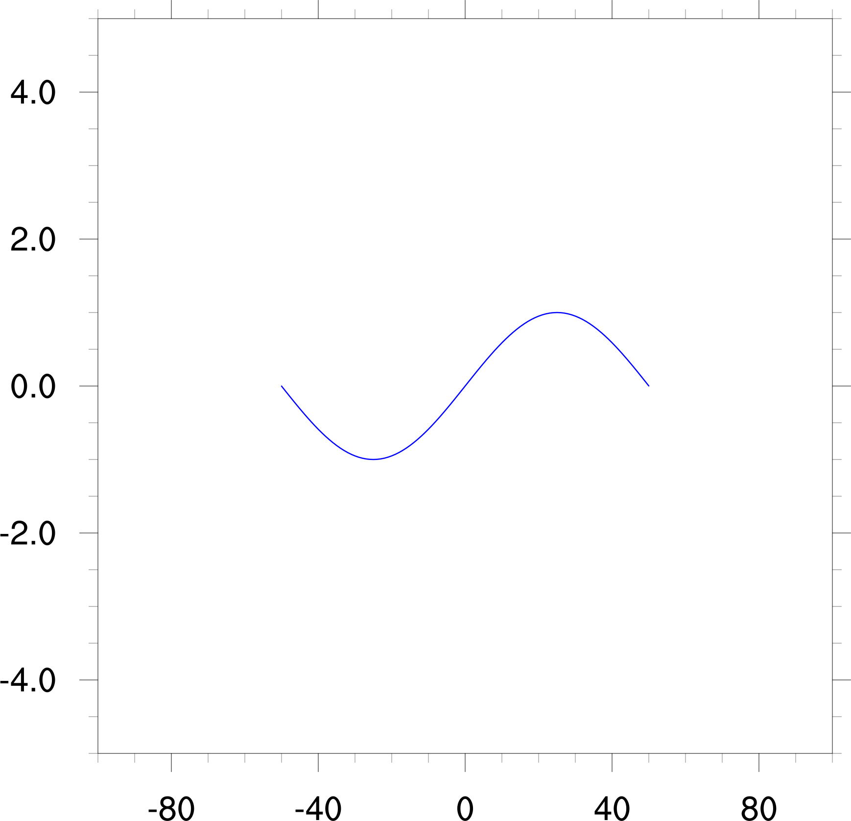
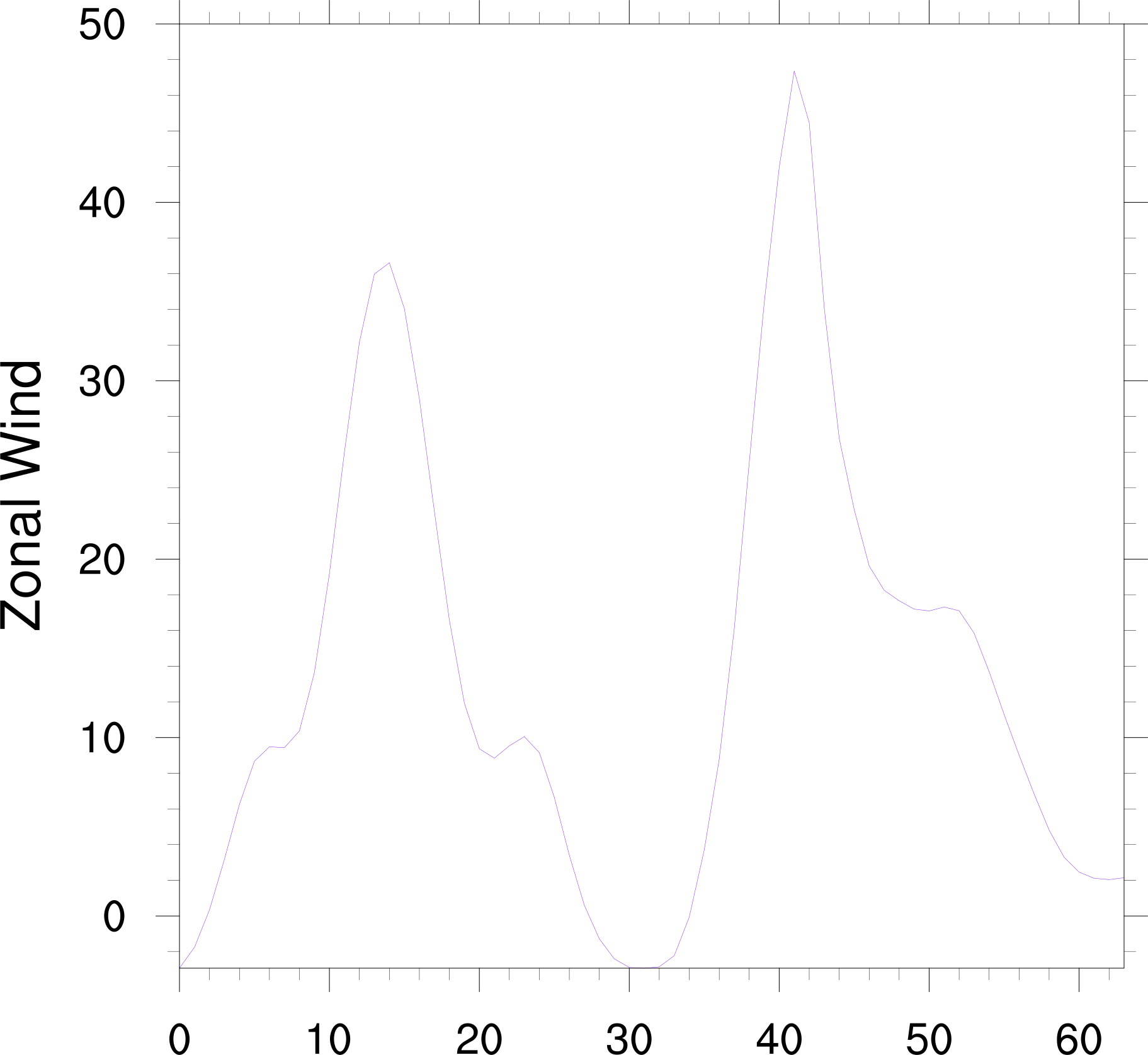
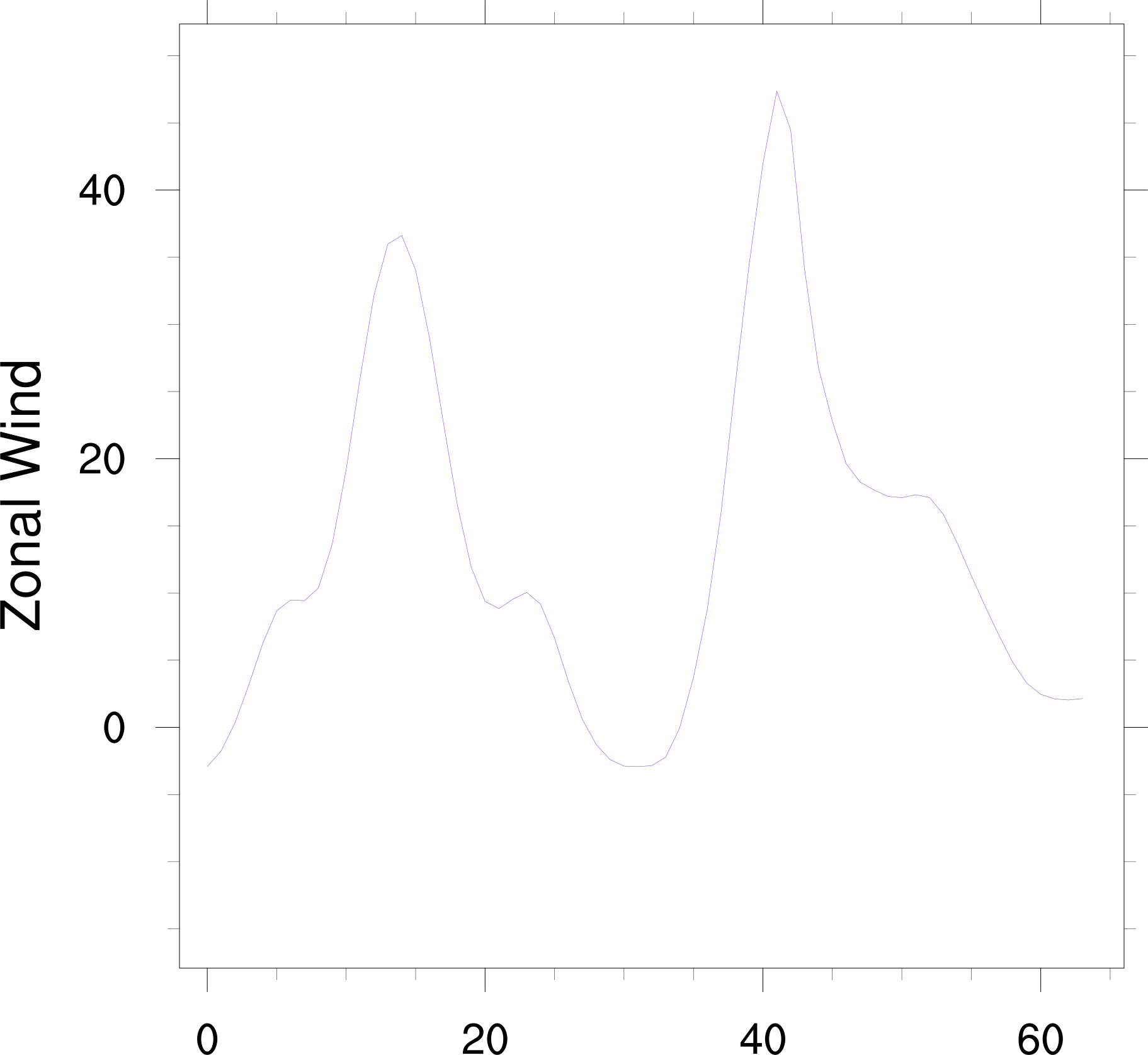
xy plots

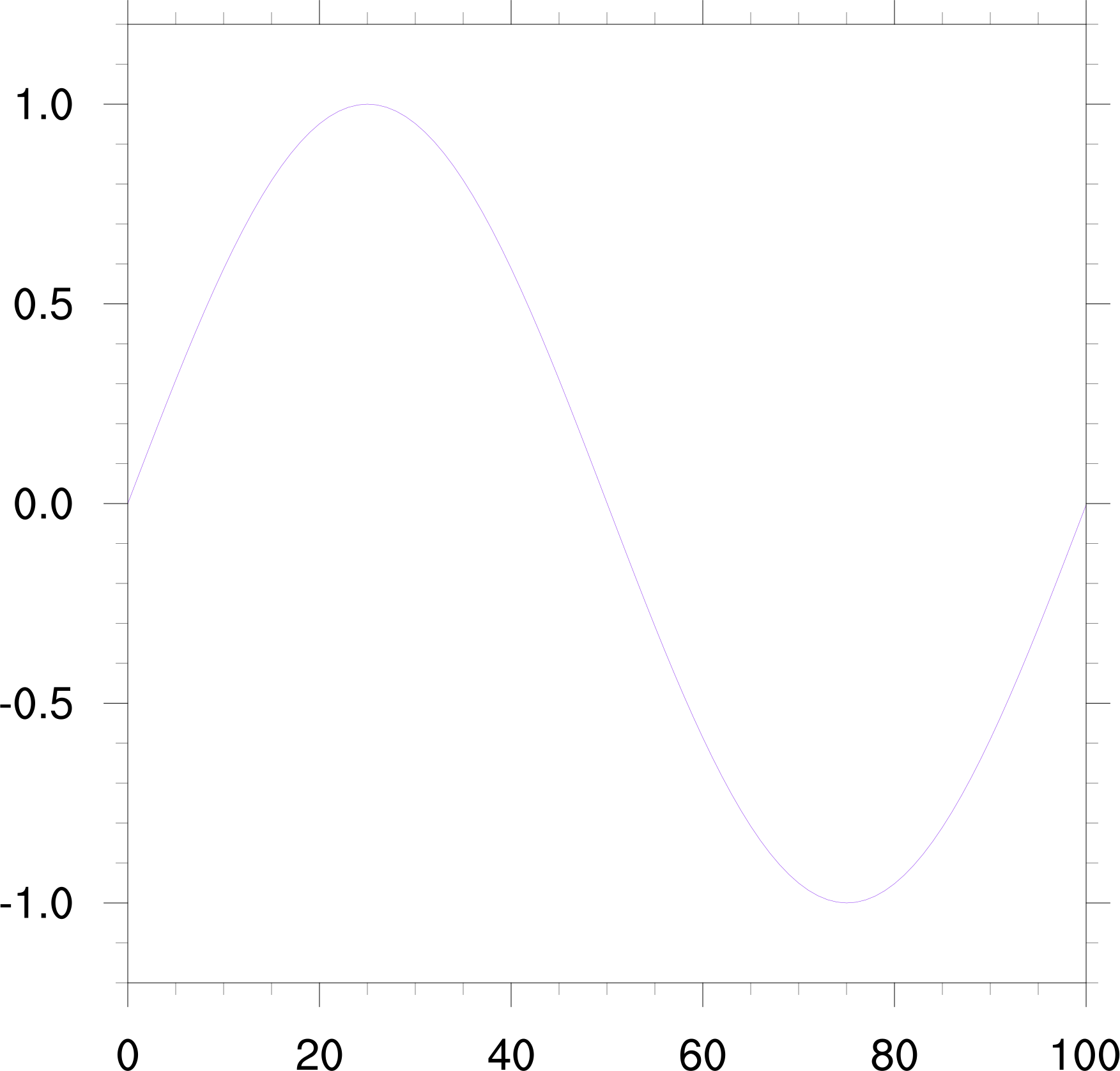
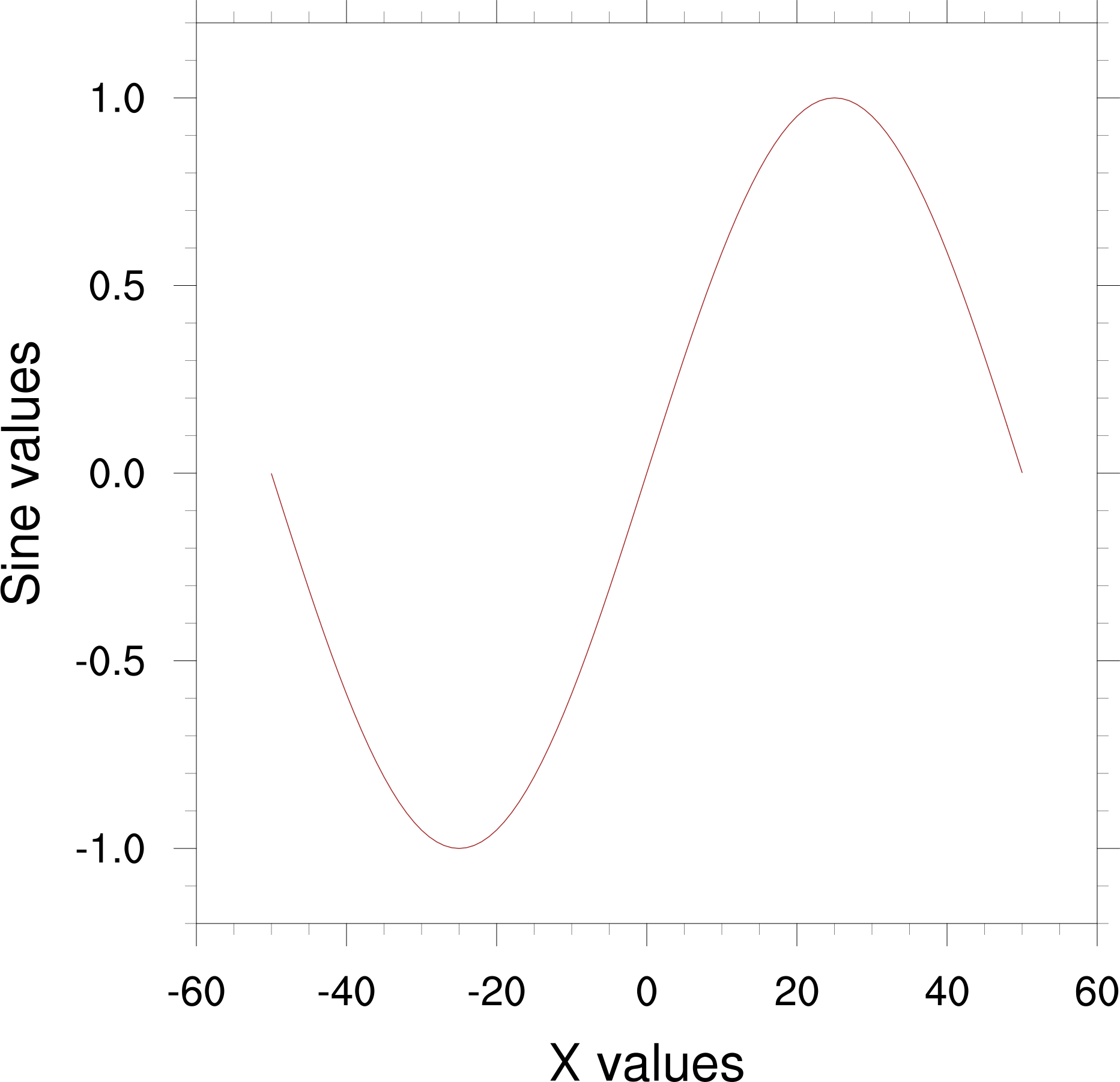
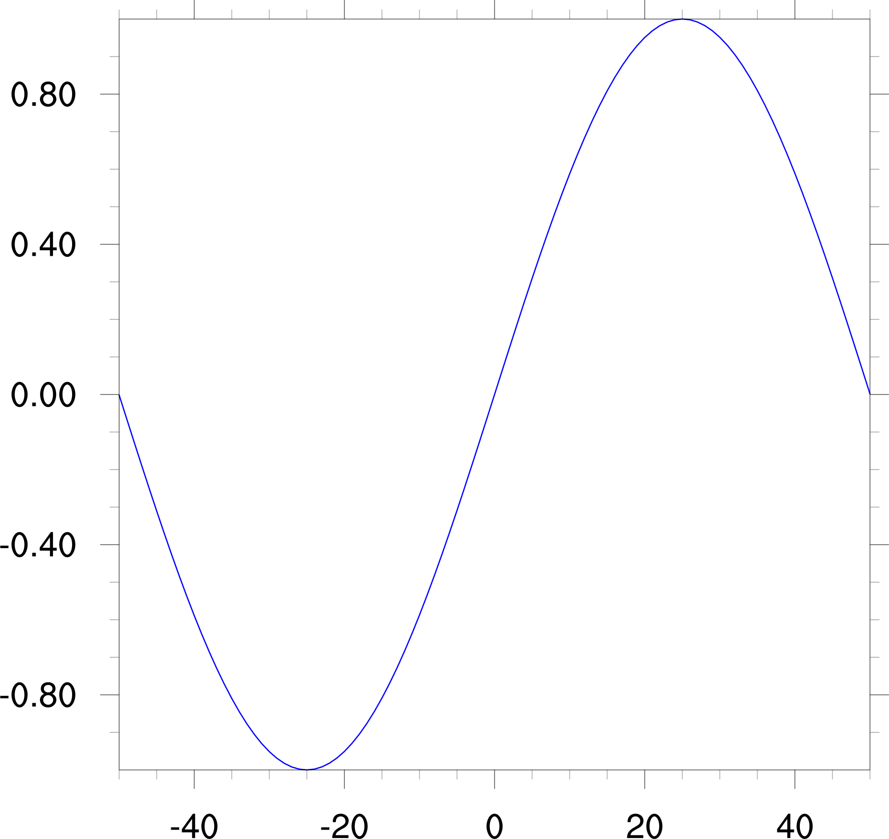
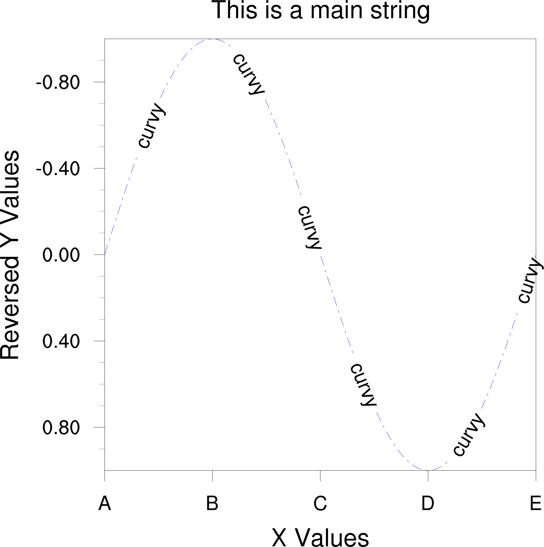
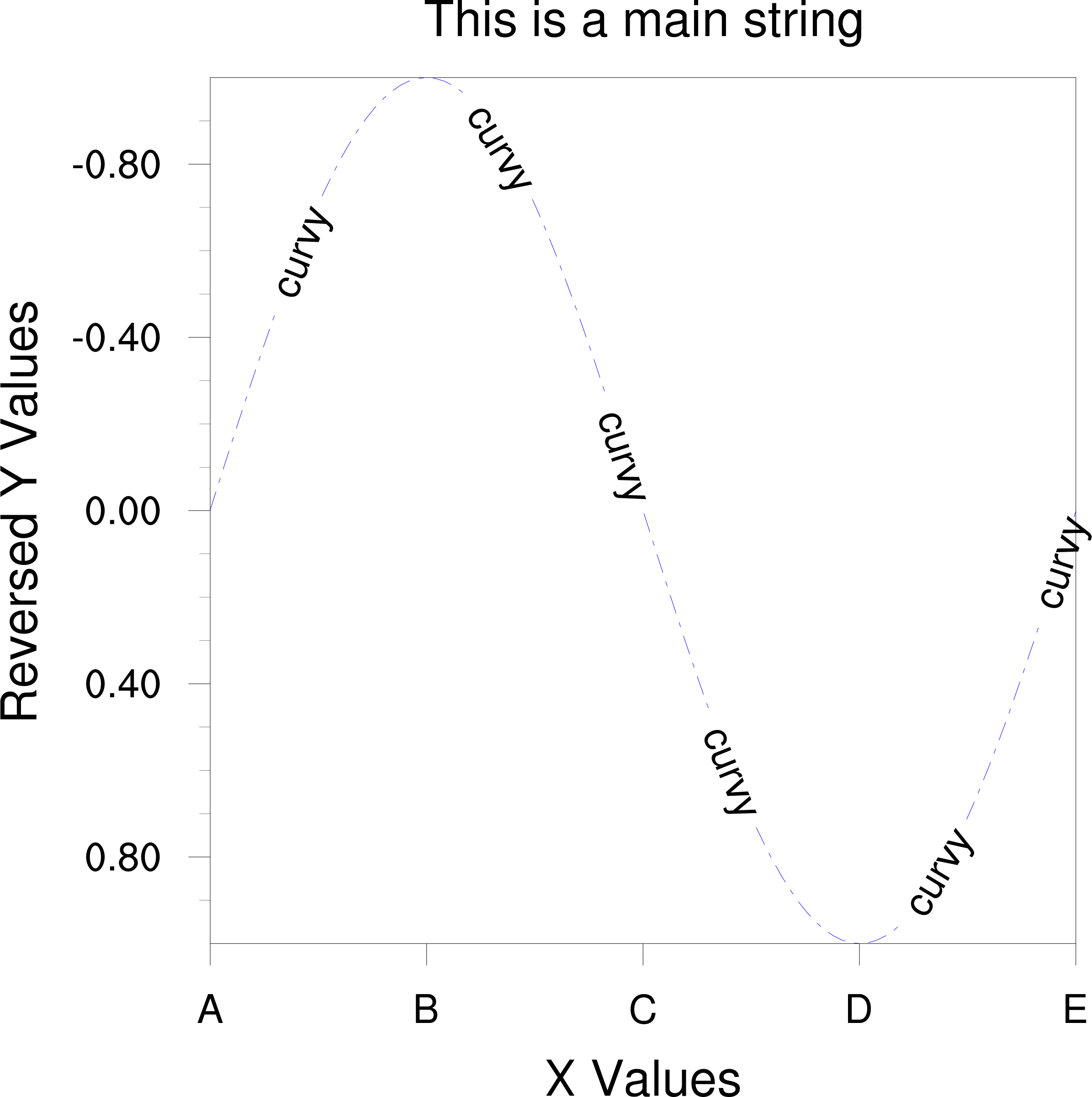
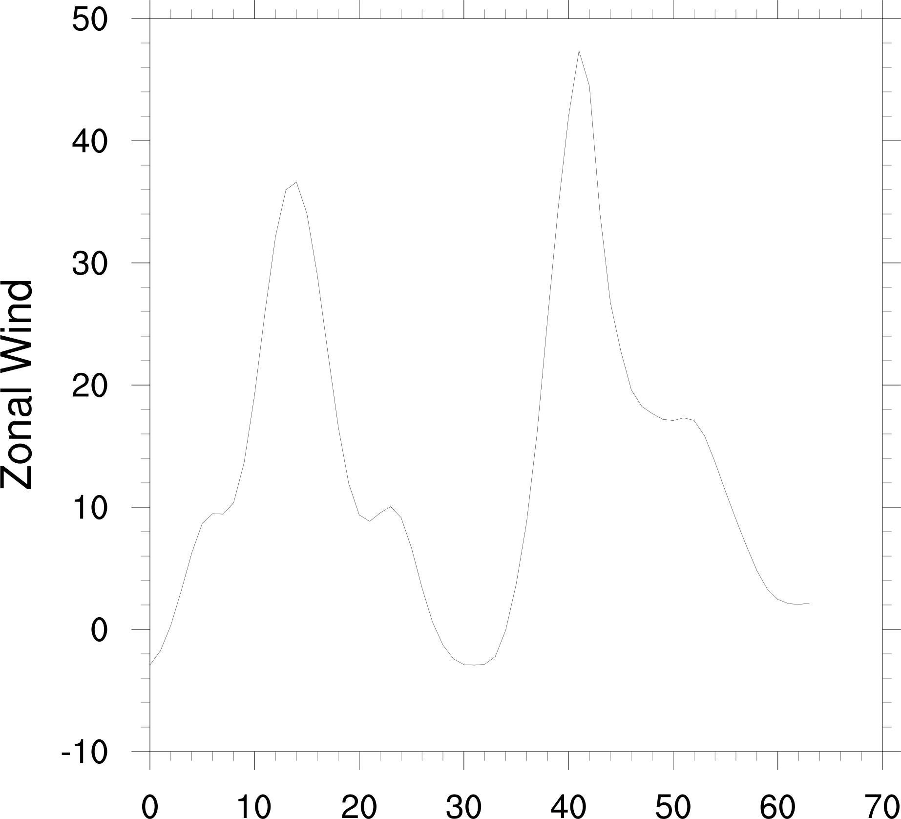
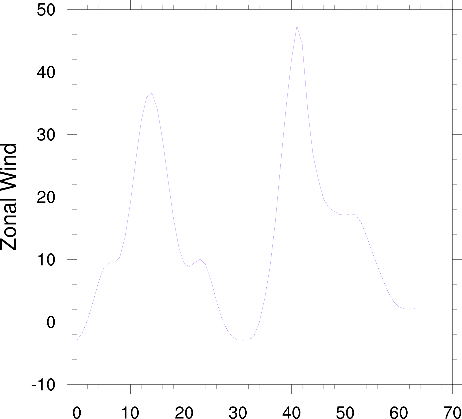
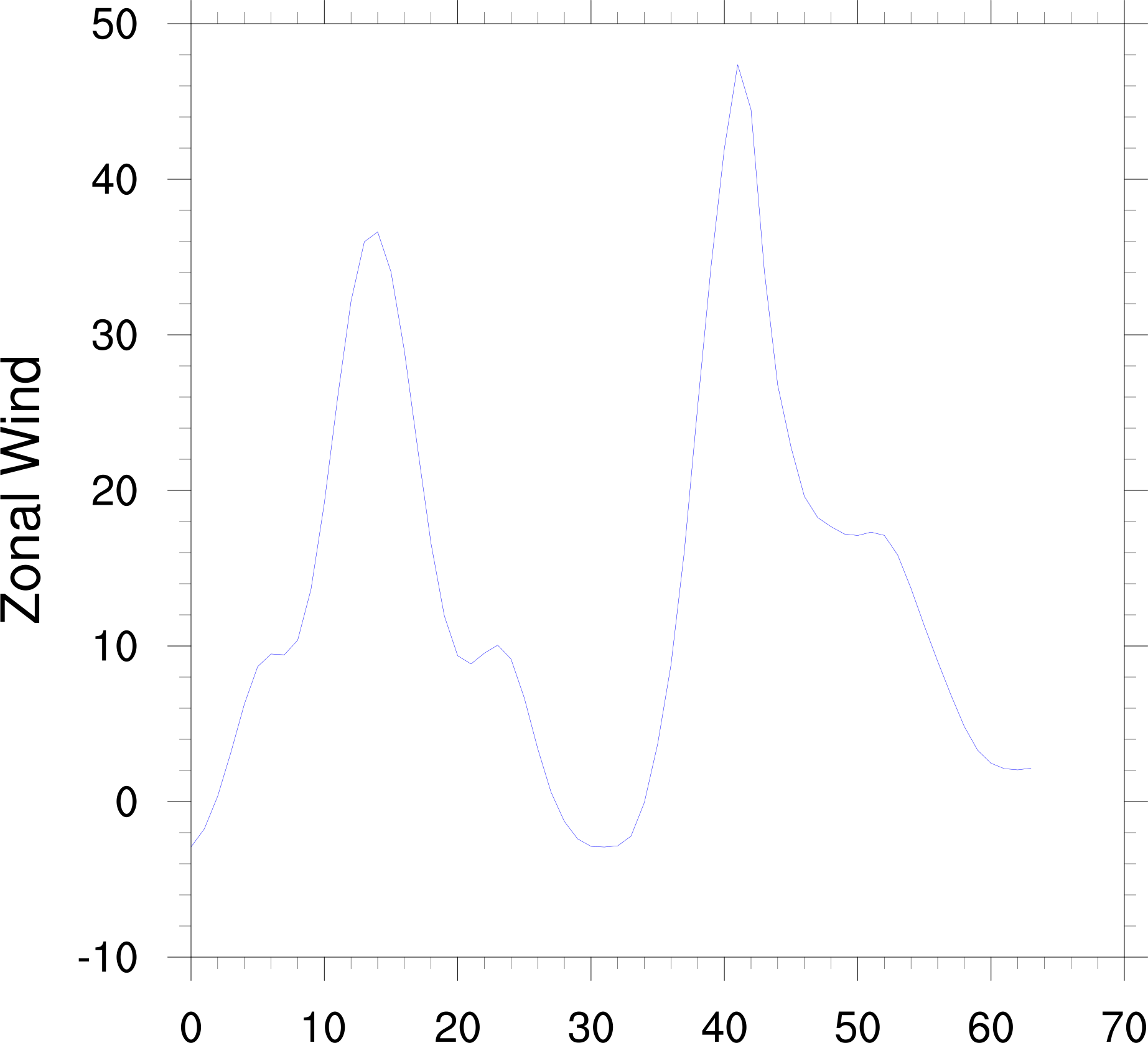
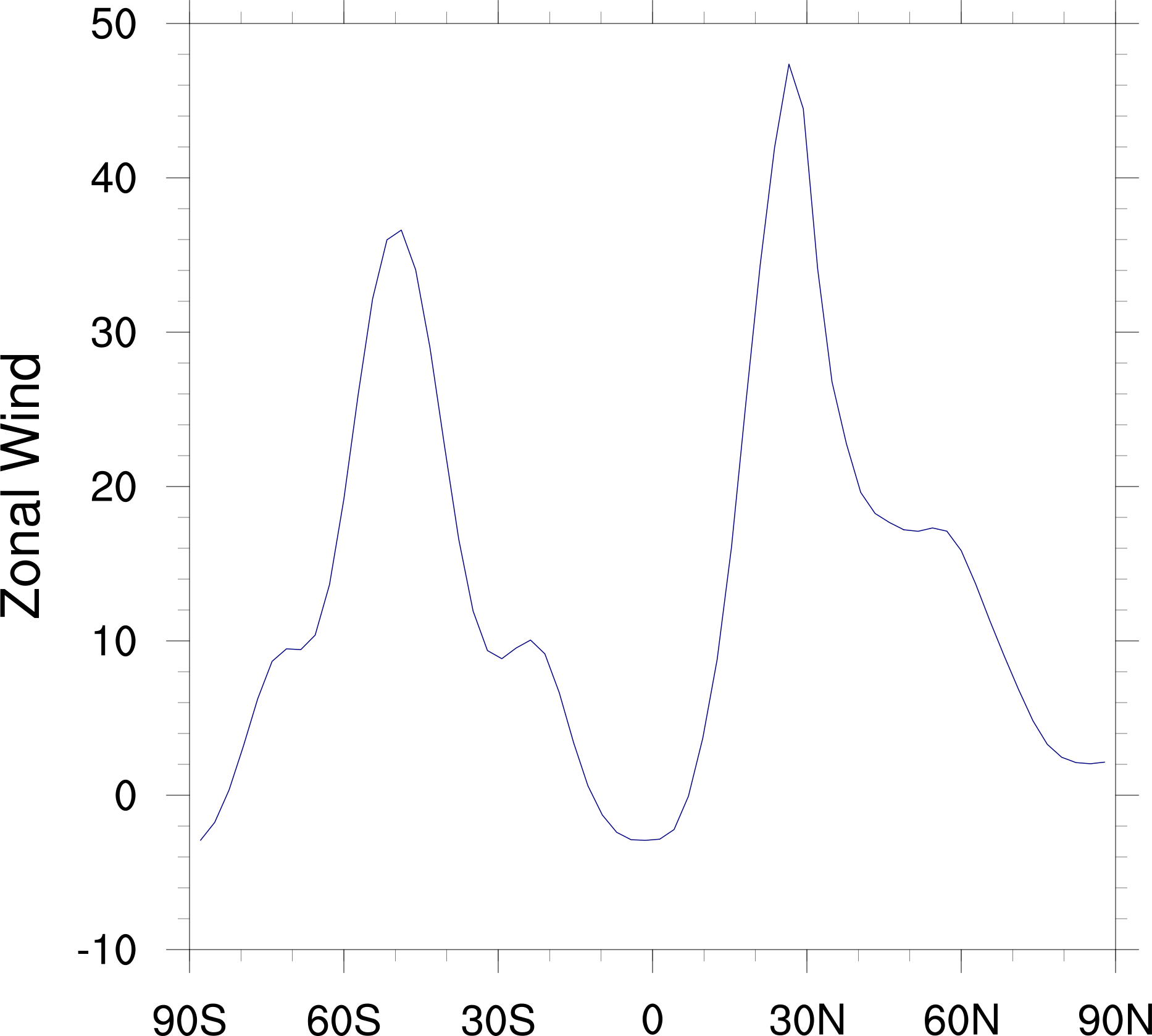
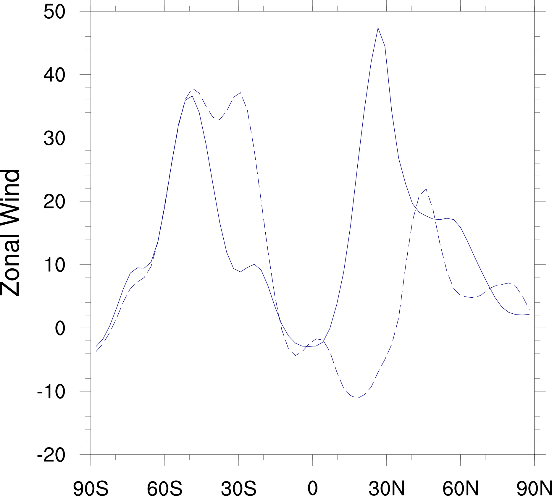
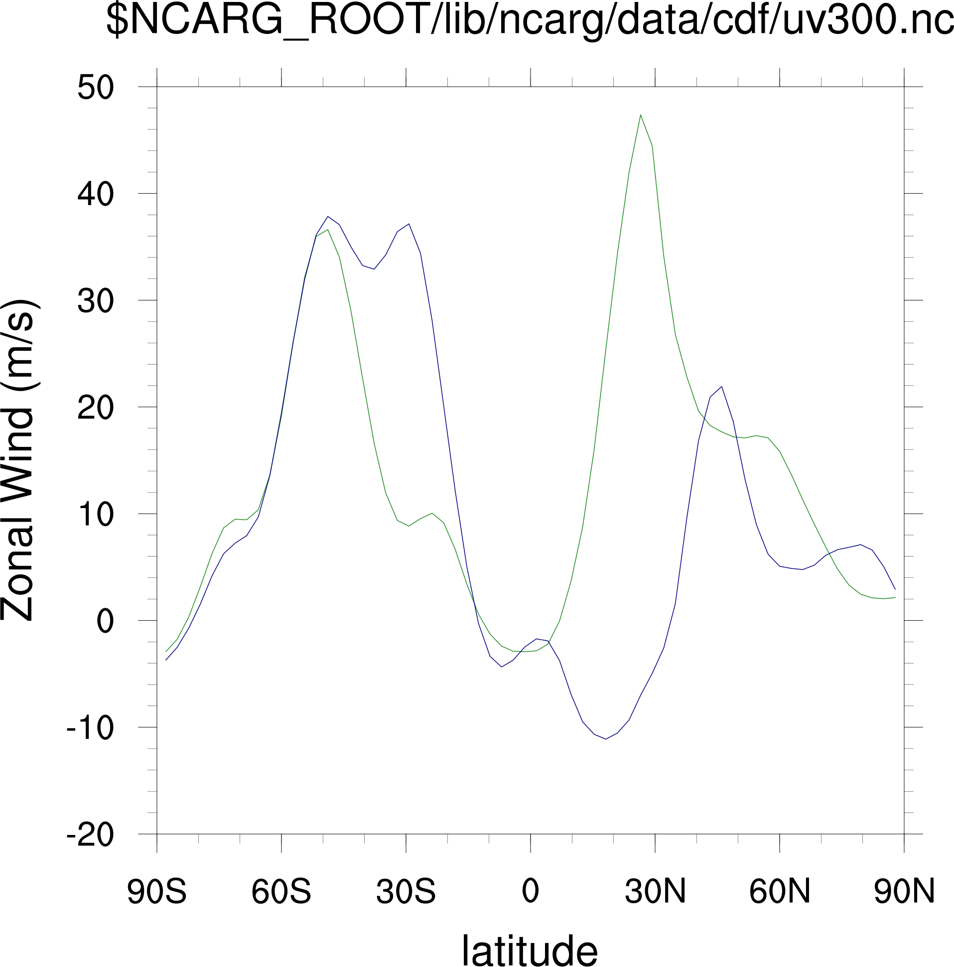
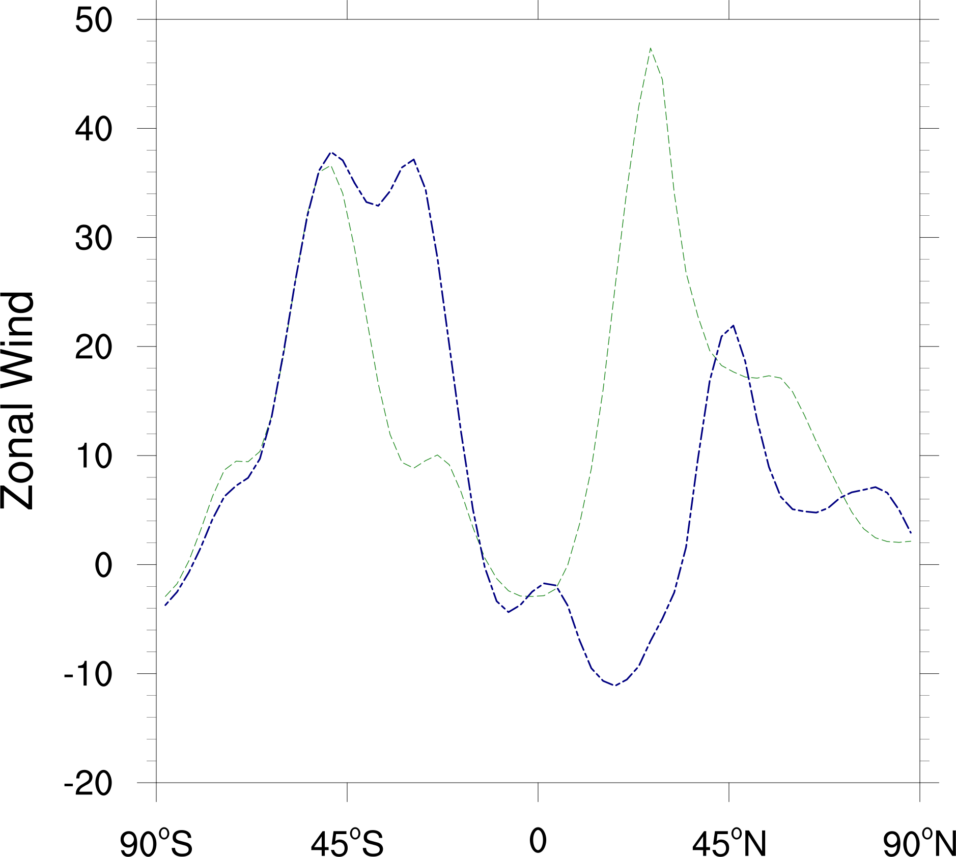
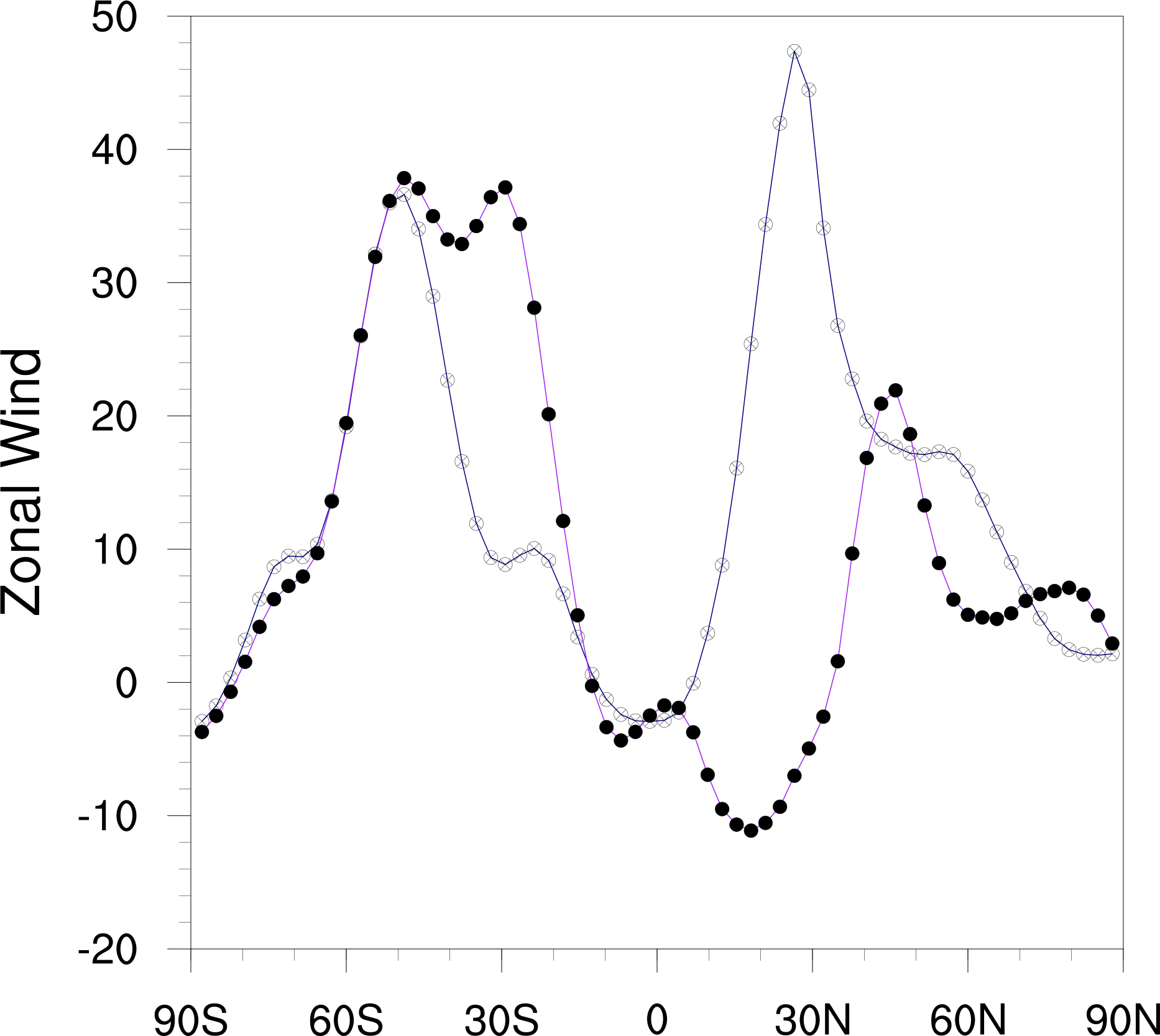
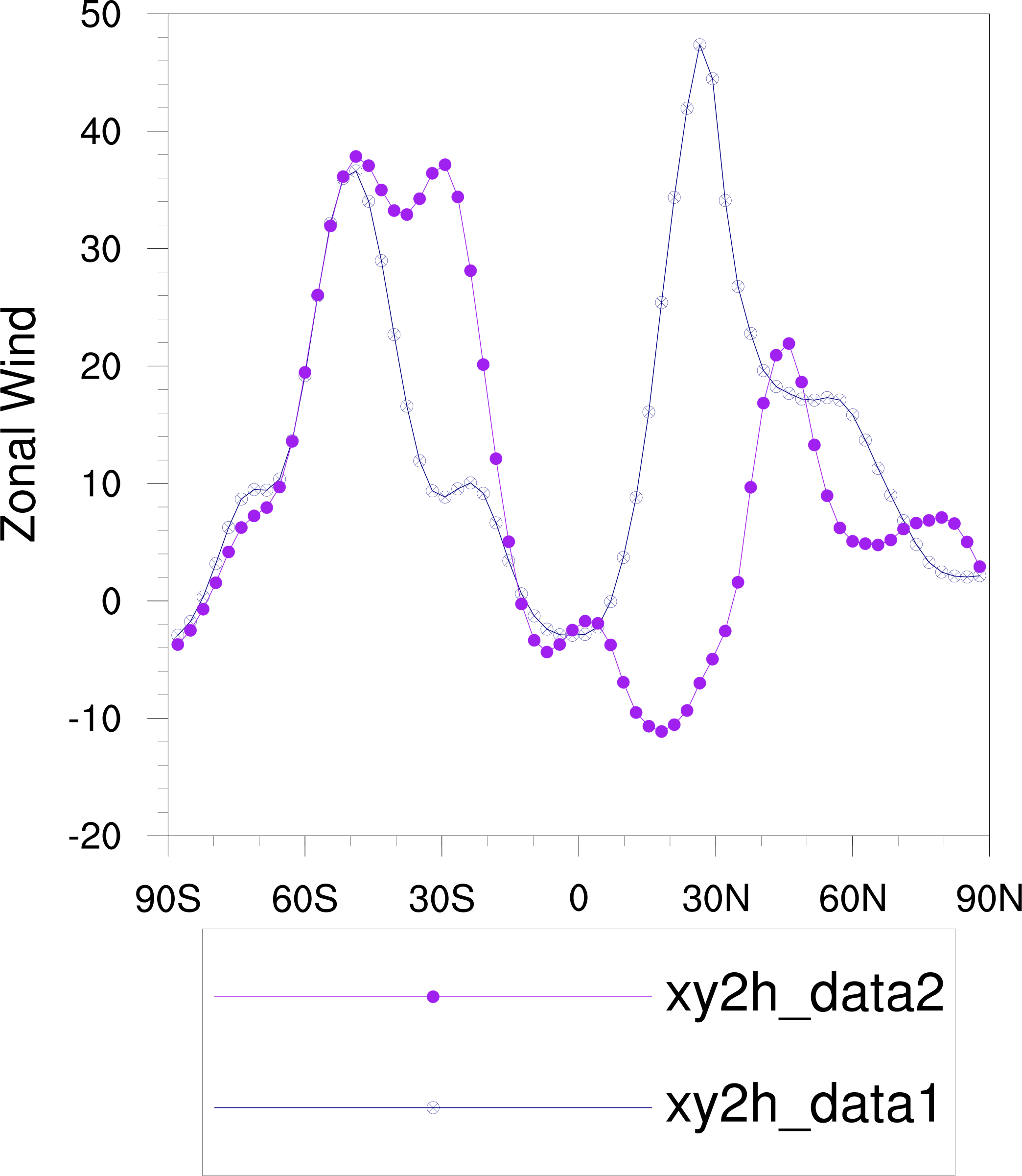
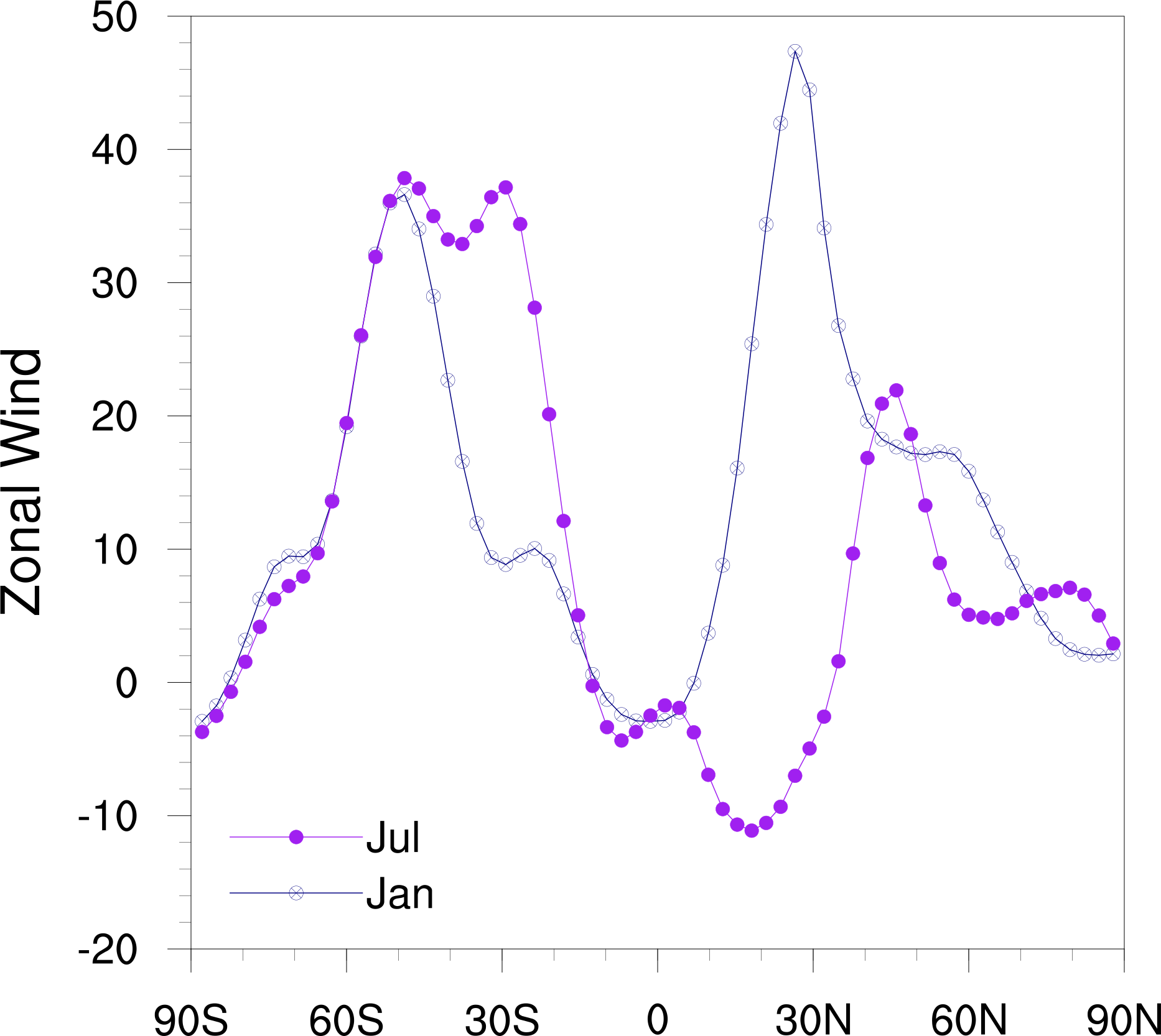
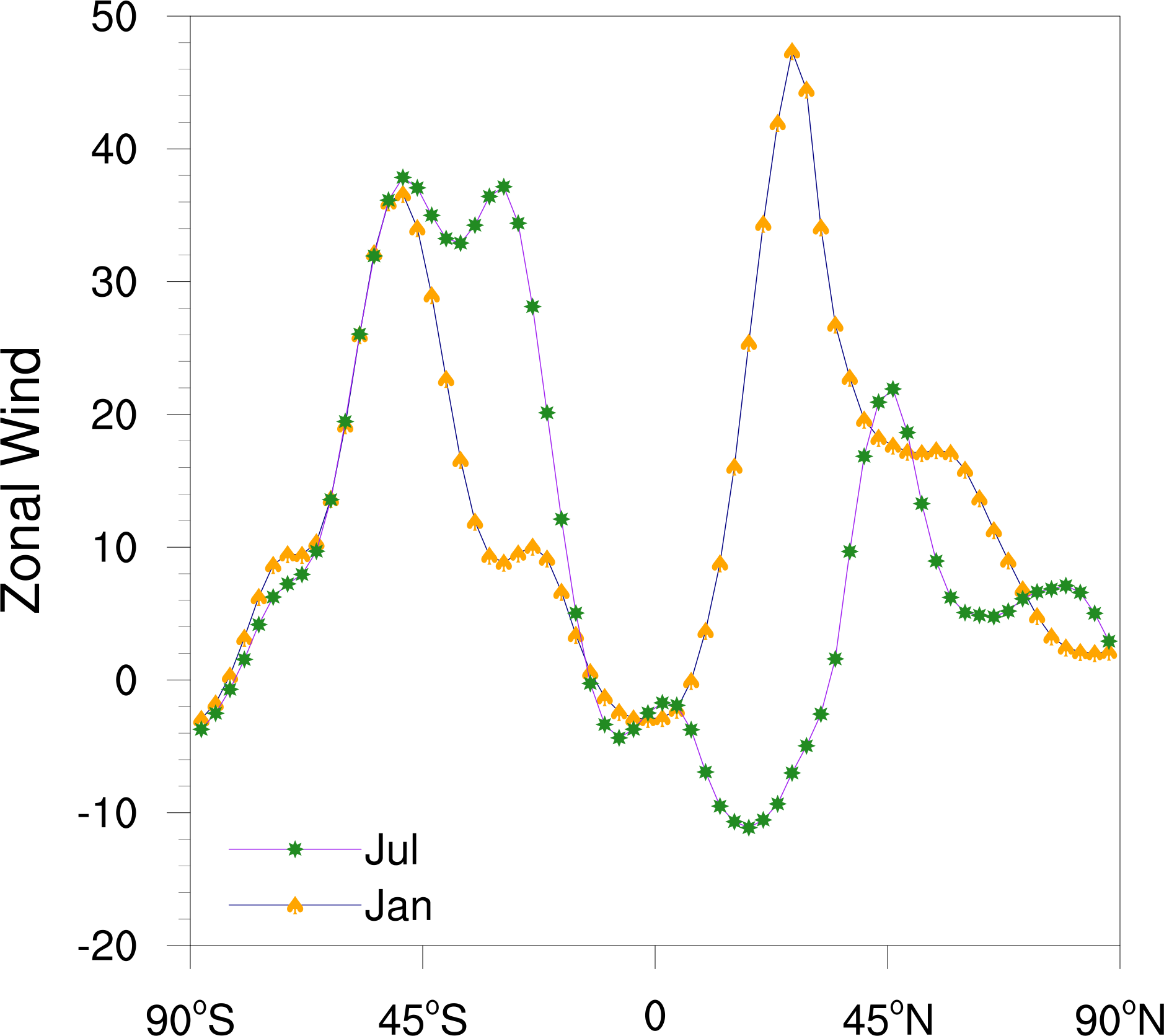
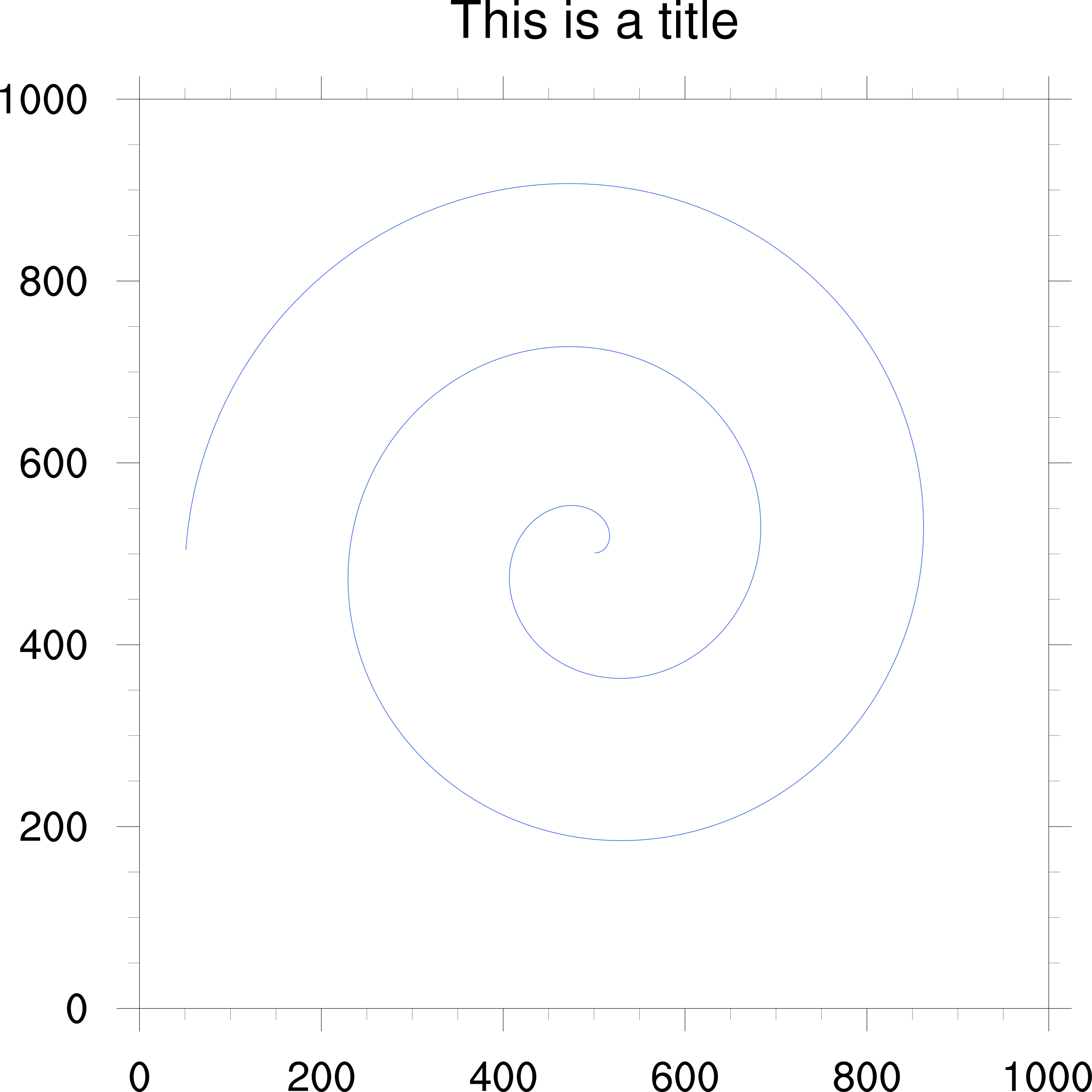
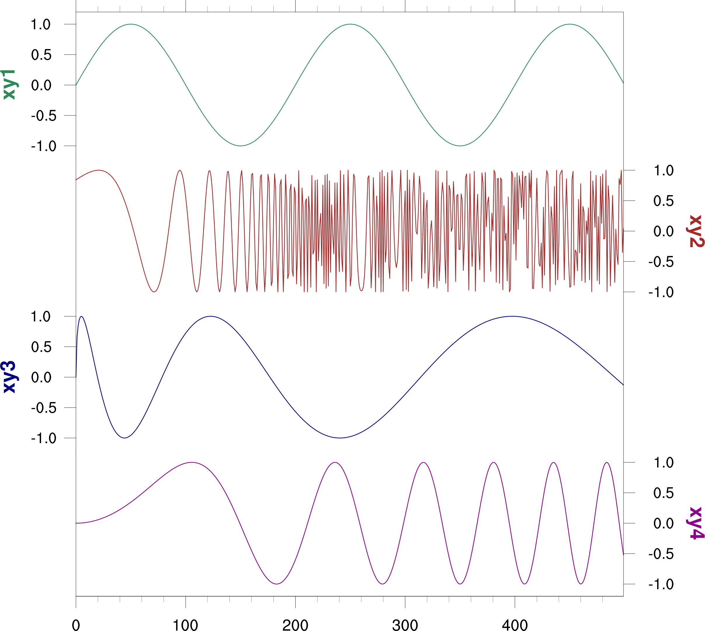
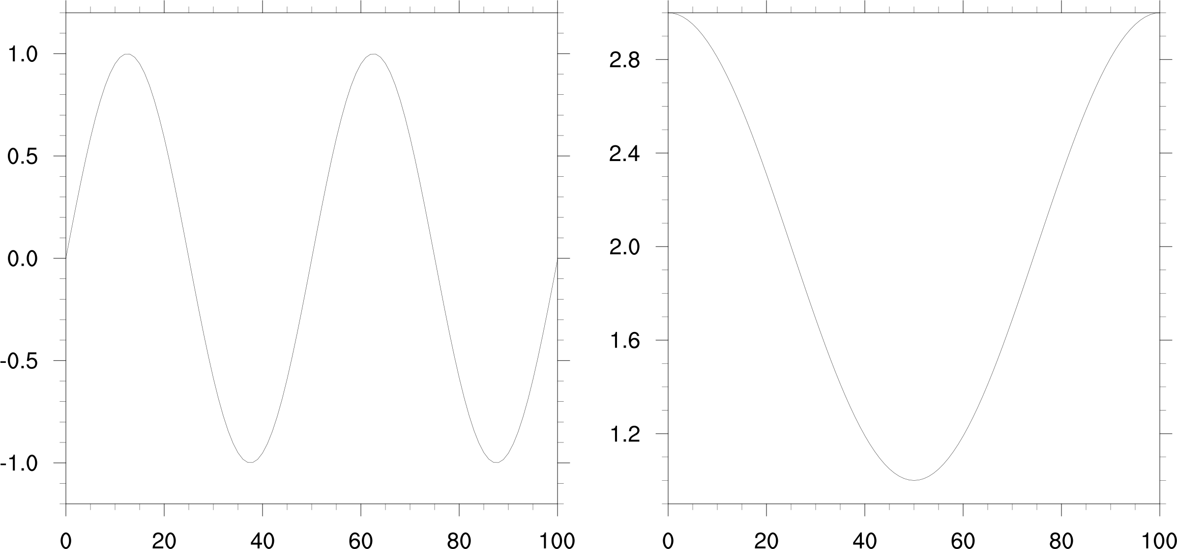
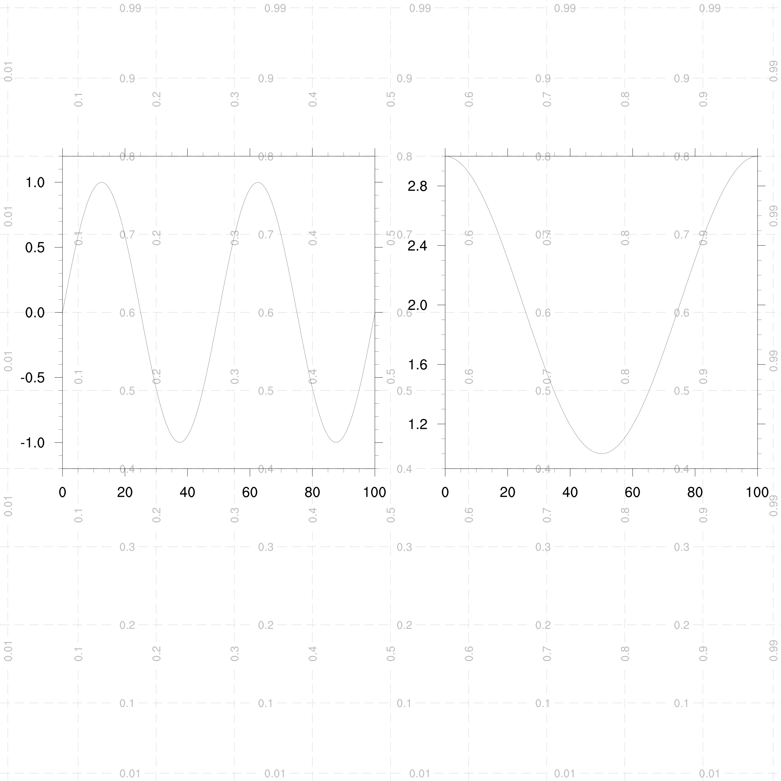
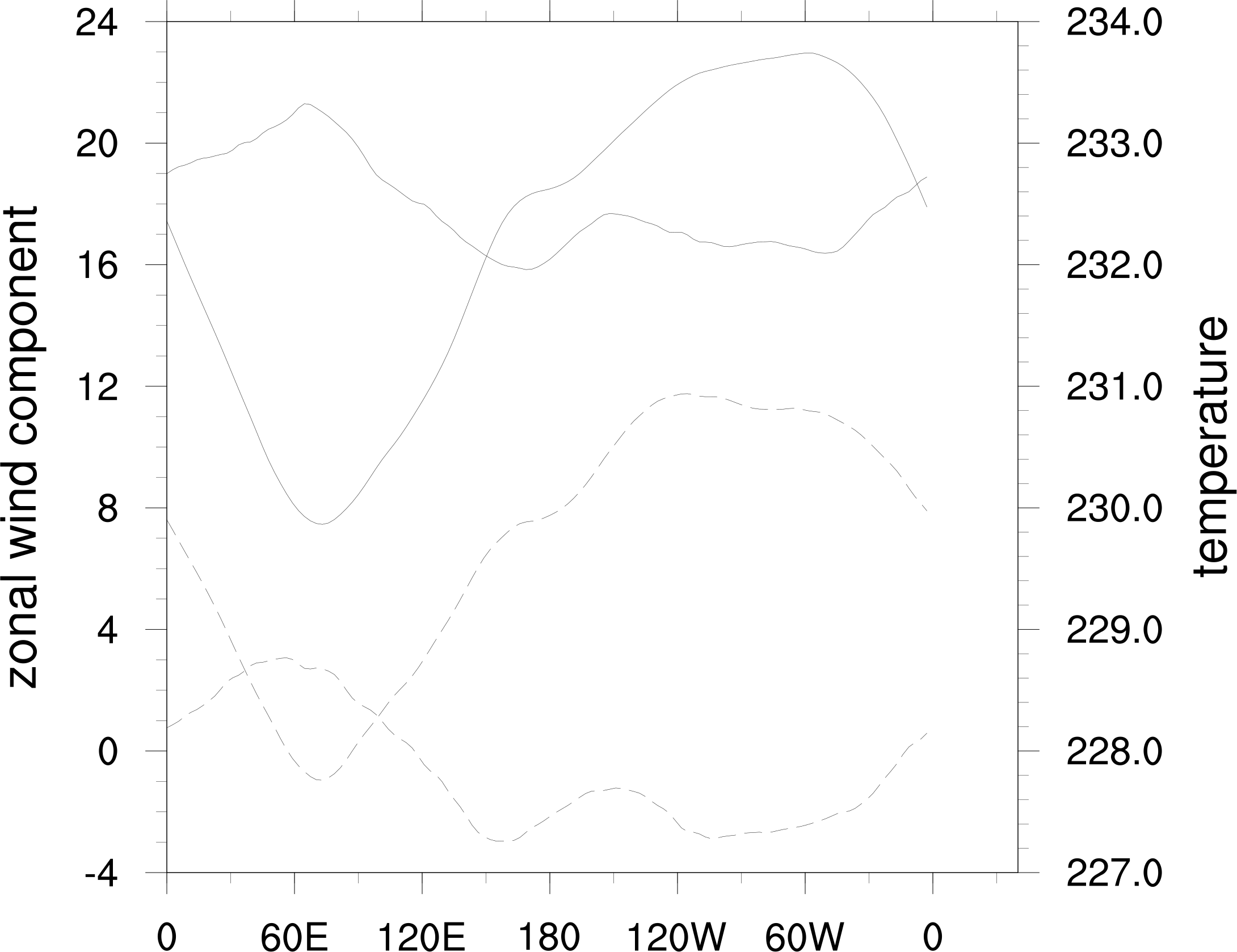
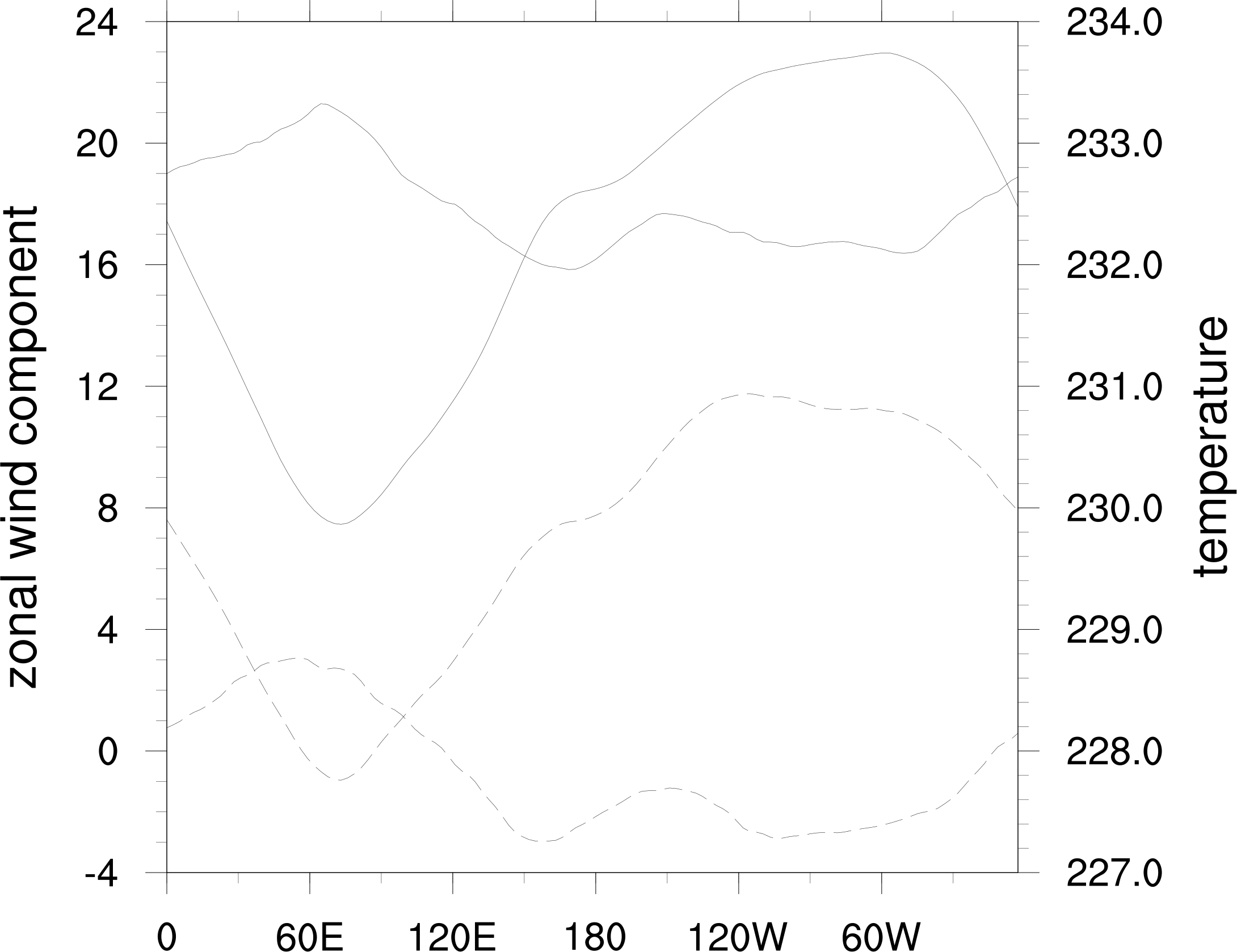
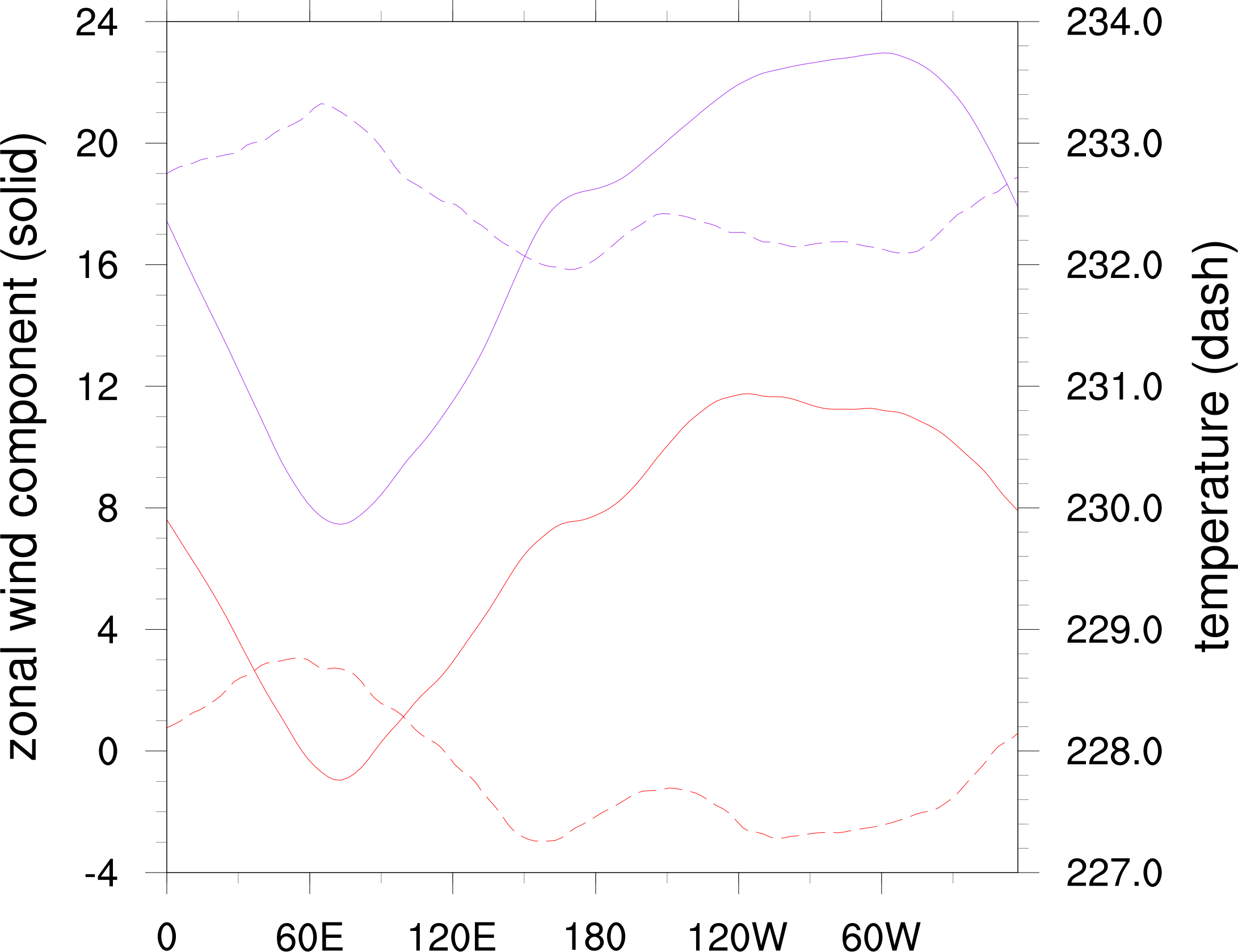
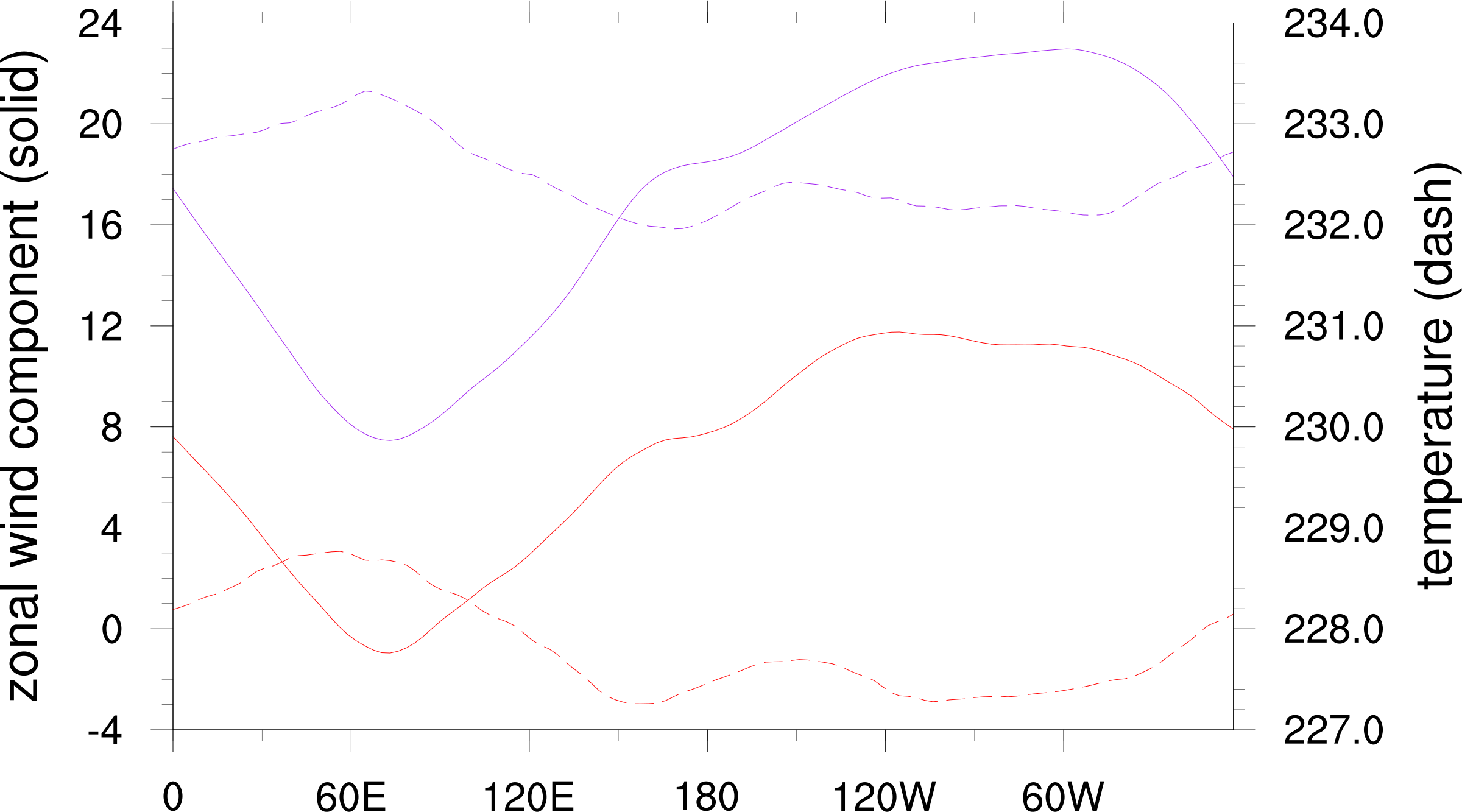
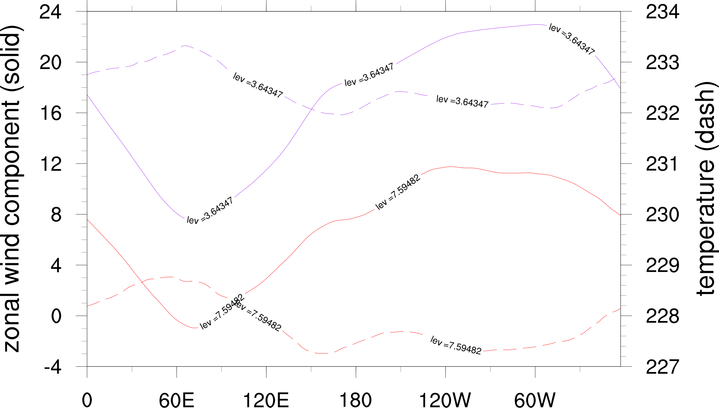
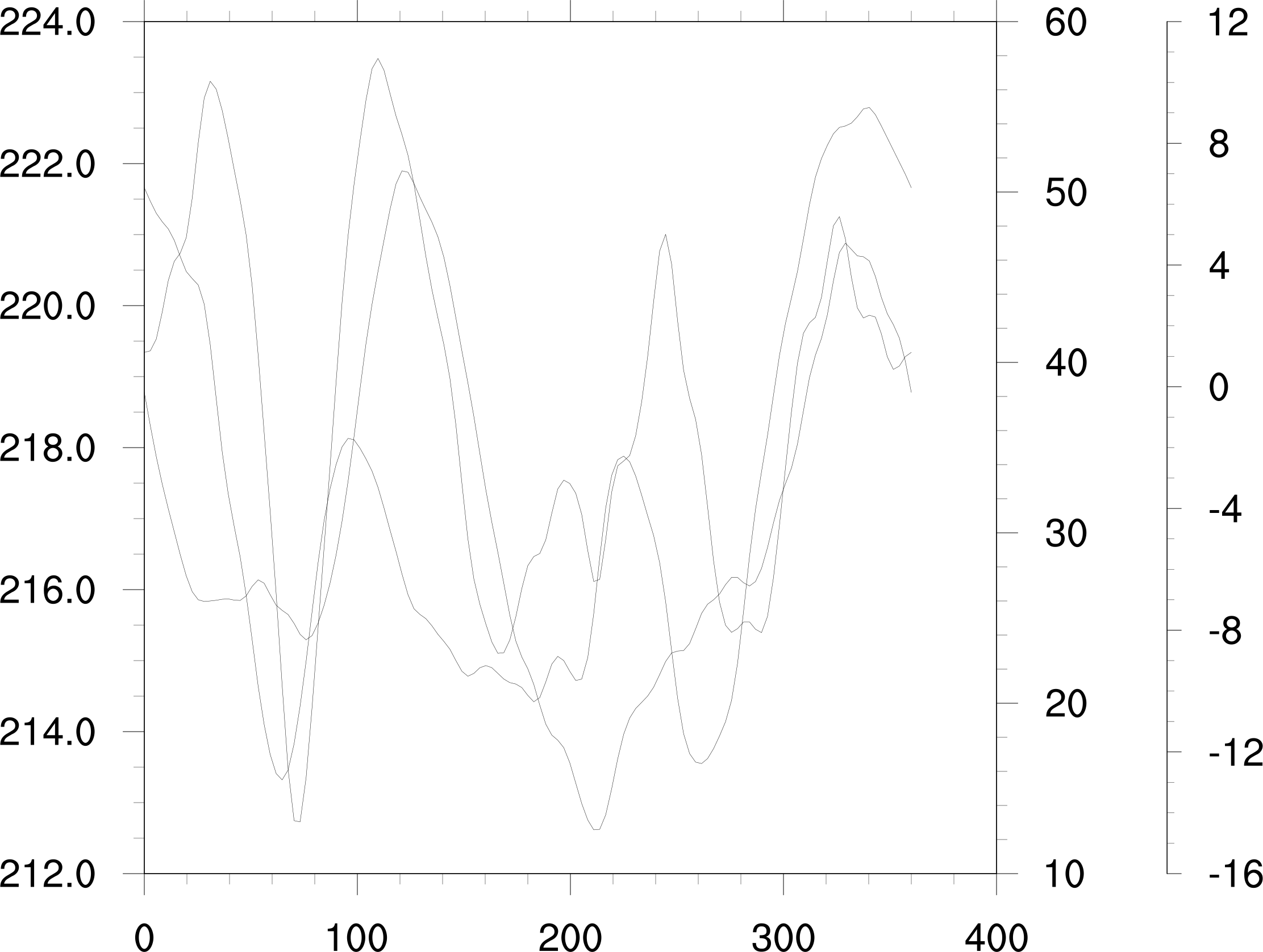
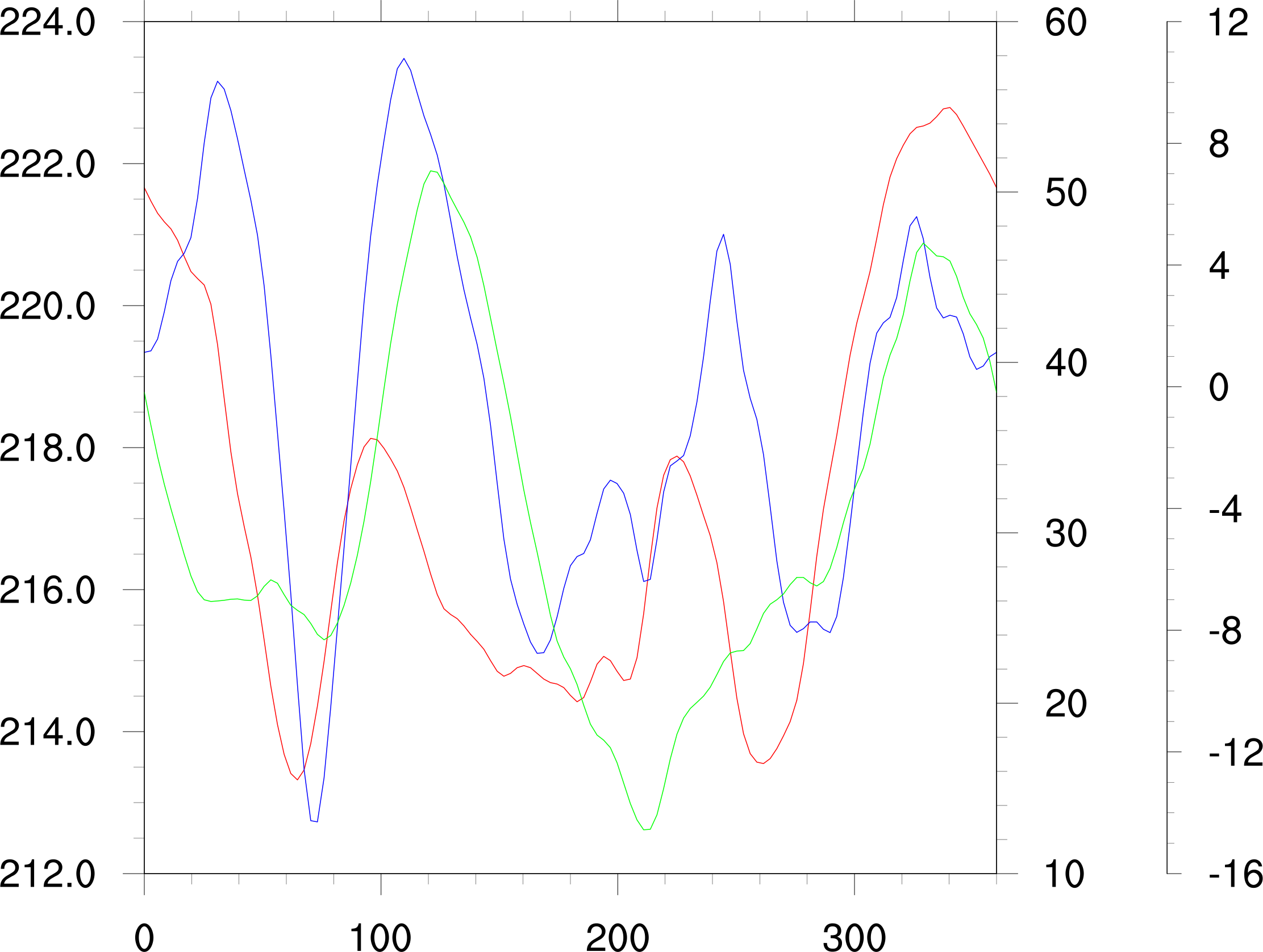
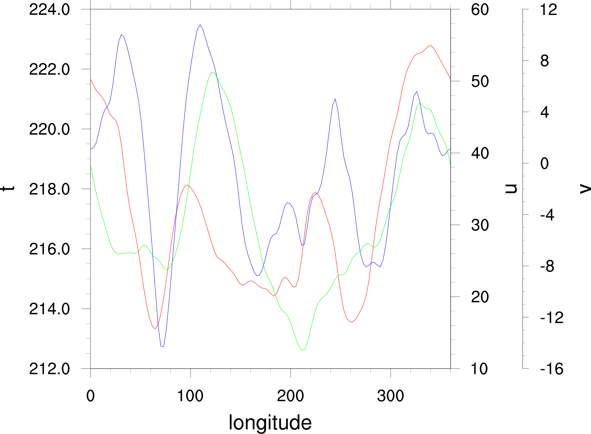
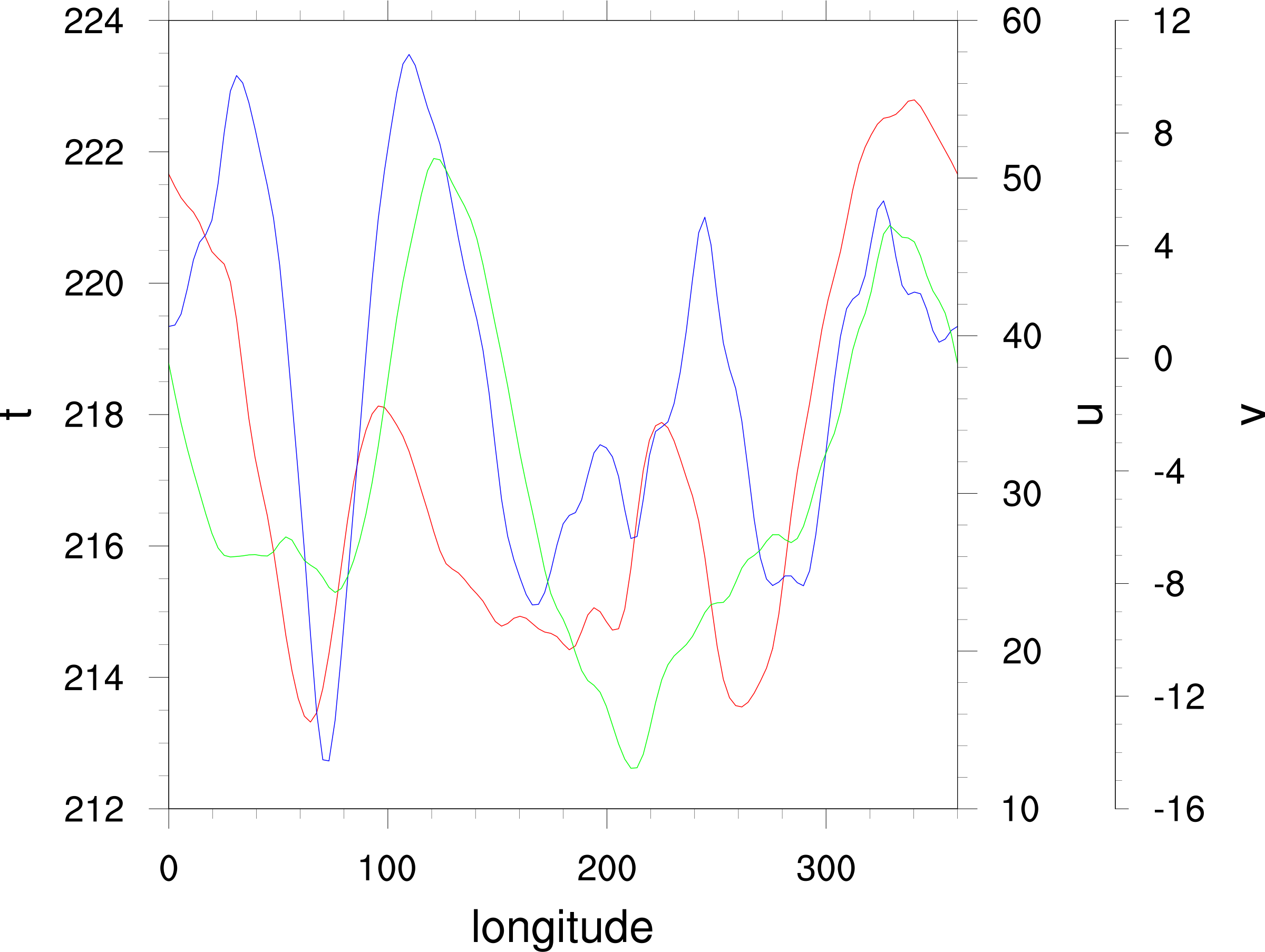
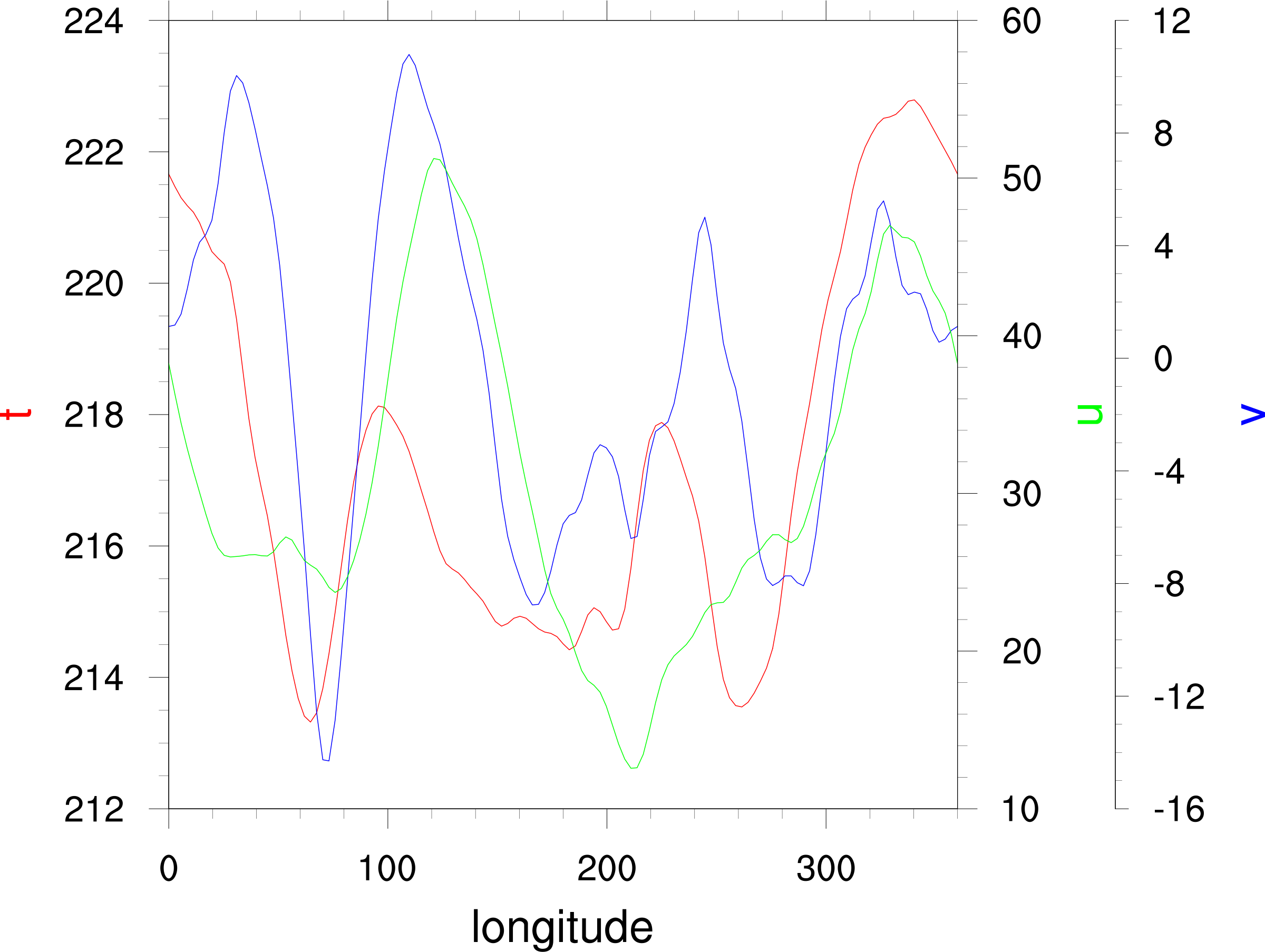
xy plots with multiple Y axes
| 
| 
| 
|
| xy4a.ncl | xy4b.ncl | xy4c.ncl | xy4d.ncl |
| 
| 
| 
|
| xy4e.ncl | xy5a.ncl | xy5b.ncl | xy5c.ncl |
| 
| ||
| xy5d.ncl | xy5e.ncl |
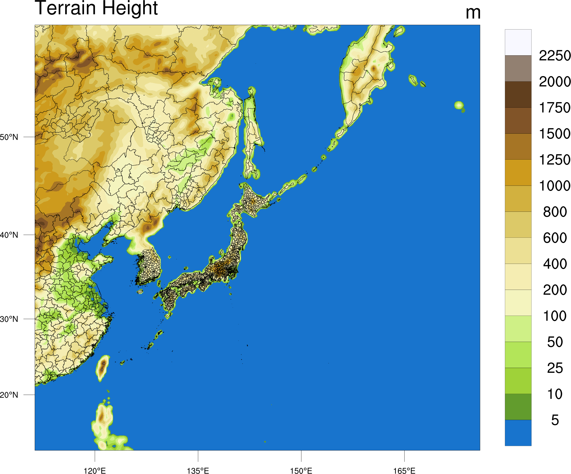
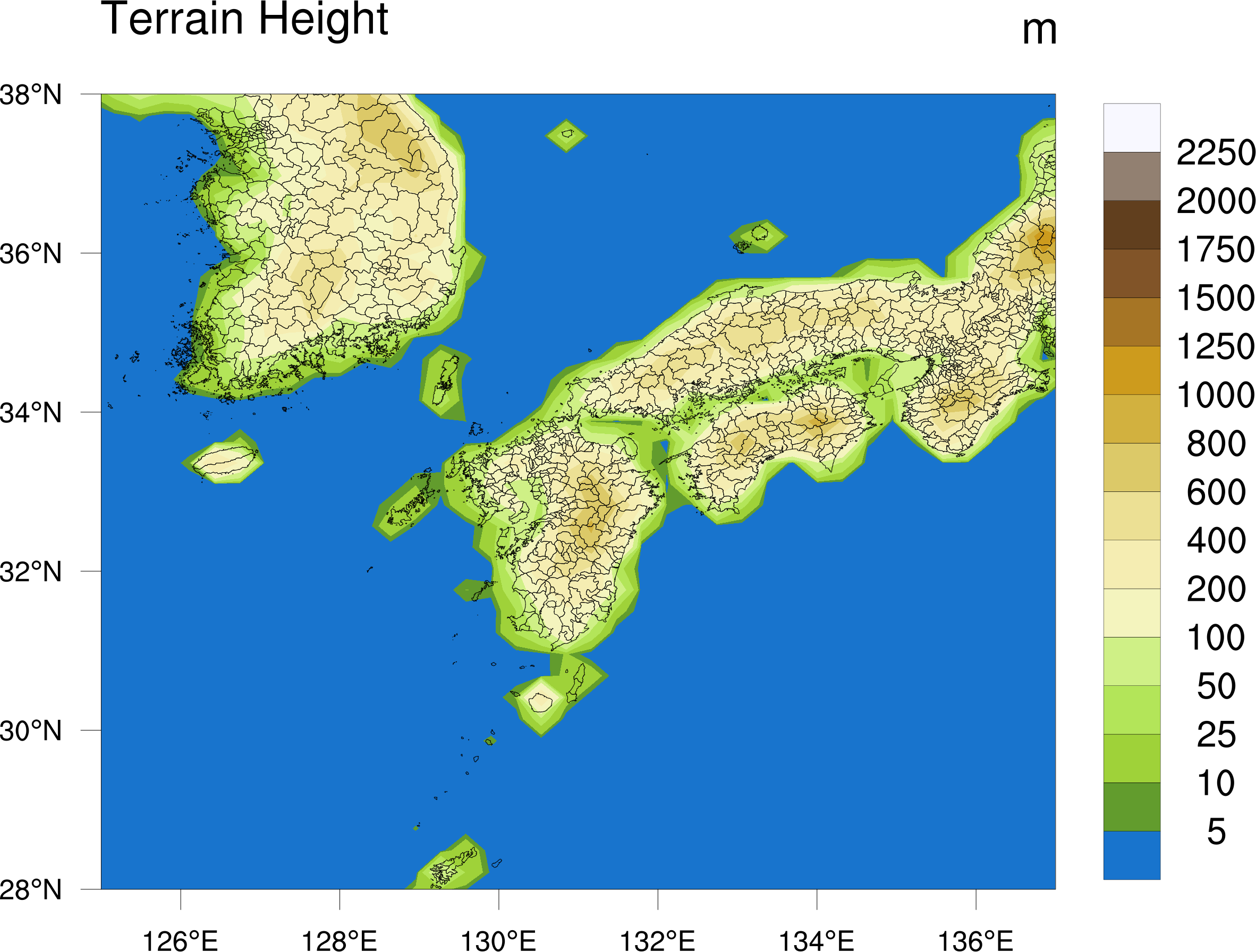
zooming in on maps (useful for looking at regional data)
|
|
|
|
|
| contour6f.ncl | contour7i.ncl | contour9f.ncl | ice.ncl |
|
|
|
|
|
| tibet.ncl | wrfgeo_gsn.ncl | wrfgsn_hgt_shapefiles_zoom.ncl | wrf_line_fill_vector_gsn.ncl |
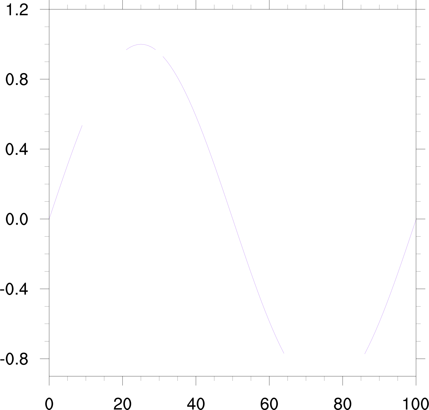
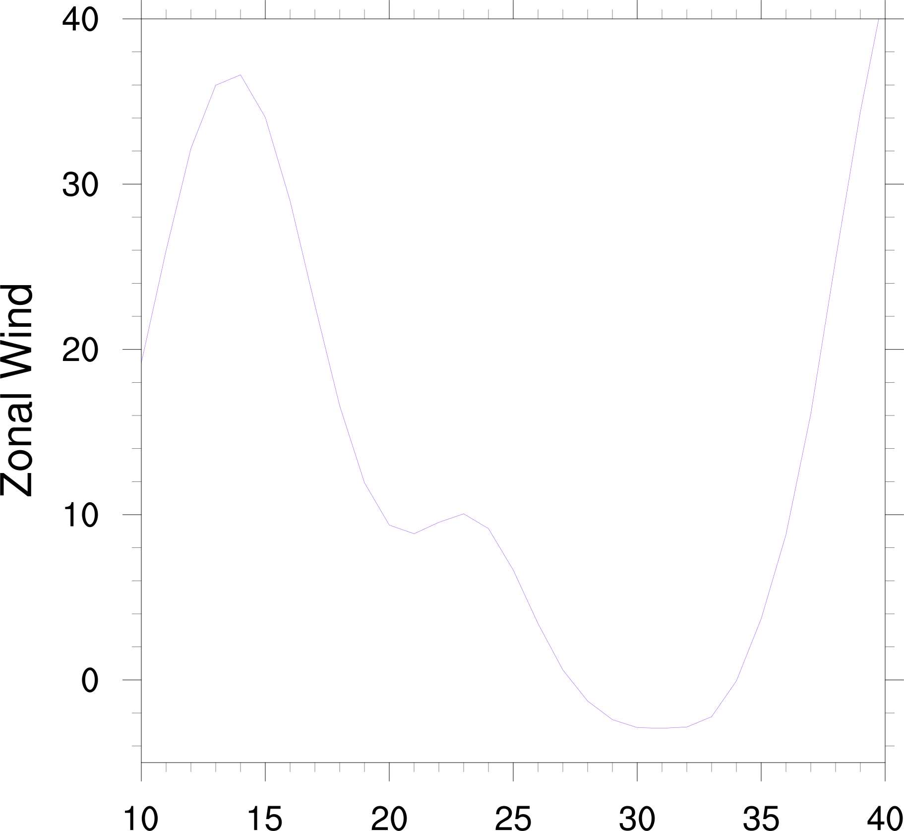
zooming in/out on xy plots
| 
| 
| 
|
| xy1d_mod1.ncl | xy1d_mod2.ncl | xy2b_zoom1.ncl | xy2b_zoom2.ncl |
| |||
| xy2b_zoom3.ncl |