NCL Home>
Application examples>
Data Analysis ||
Data files for some examples
Example pages containing:
tips |
resources |
functions/procedures
NCL: Bootstrapping and Resampling
Bootstrapping
is a statistical method that uses data resampling with replacement
(see:
generate_sample_indices)
to estimate the robust properties of nearly any statistic. Most commonly, these include
standard errors and confidence intervals of a population parameter like a mean, median,
correlation coefficient or regression coefficient. Bootstrapping statistics has two
attractive attributes:
- It is particularly useful when dealing with small sample sizes.
- It makes no apriori assumption about the distribution of the sample data.
References:
Computer Intensive Methods in Statistics
   P. Diaconis and B. Efron
   Scientific American (1983), 248:116-130
   doi:10.1038/scientificamerican0583-116
   http://www.nature.com/scientificamerican/journal/v248/n5/pdf/scientificamerican0583-116.pdf

An Introduction to the Bootstrap
   B. Efron and R.J. Tibshirani, Chapman and Hall (1993)

Statistical methods for the analysis of simulated and observed climate data
   Barbara Hennemuth et al (2013)
   Applied in projects and institutions dealing with climate change impact and adaptation
    CSC Report 13

Bootstrap Methods and Permutation Tests: Companion Chapter 18 to the Practice of Business Statistics
   Hesterberg, T. et al (2003)
   http://statweb.stanford.edu/~tibs/stat315a/Supplements/bootstrap.pdf

Climate Time Series Analysis: Classical Statistical and Bootstrap Methods
   M. Mudelsee (2014) Second edition. Springer, Cham Heidelberg New York Dordrecht London
   ISBN: 978-3-319-04449-1, e-ISBN: 978-3-319-04450-7
   doi: 10.1007/978-3-319-04450-7
   xxxii + 454 pp; Atmospheric and Oceanographic Sciences Library, Vol. 51
NCL (6.4.0 ) currently has four bootstrap statistic functions and one bootstrap utility function:
Some NCL bootstrap functions allow for
subsampling (
n<N) and for sequential blocks (sequences) of values.
More involved sampling strategies may require custom codes. A user could extract
one of the above core functions from the contributed.ncl library and modify as needed.
Several of the NCL examples use two 'law school' data sets from Efron and Tibshirani (1993).
These contain LSAT (Law School Admission Test) scores and subsequent GPAs (Grade Point Averages).
One data set,
law_school_82.txt, contains the
LSAT and GPA for 82 law schools; the second data set,
law_school_15.txt contains a random sample
from 15 of the 82 schools. The reason for using these is that WWW-accessible results using both
R and
Matlab_1 and
Matlab_2
are readily available for comparison purposes.
See:
regression Example 7
for a visualization of these files.
 resampling_1.ncl
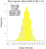
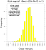
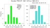
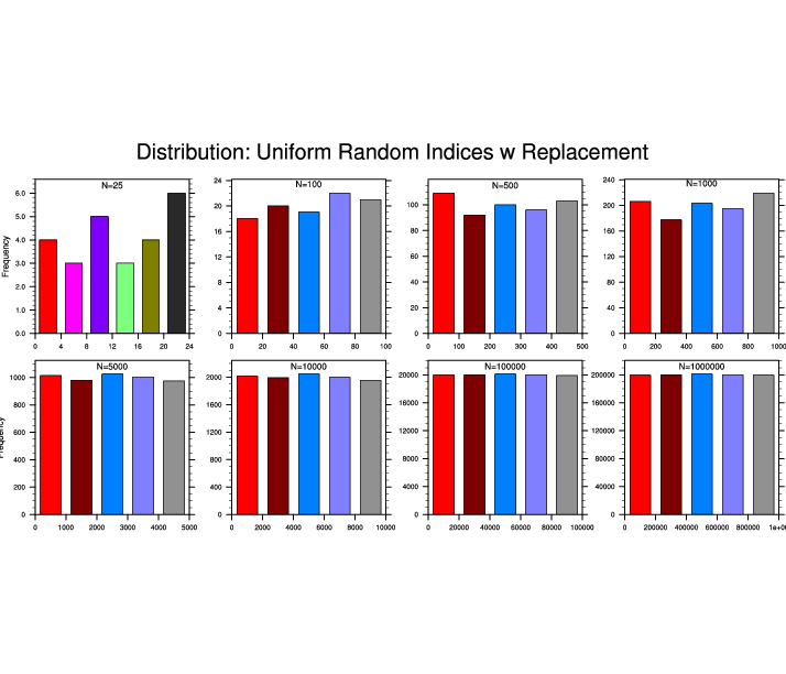
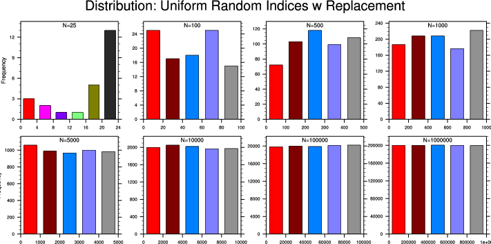
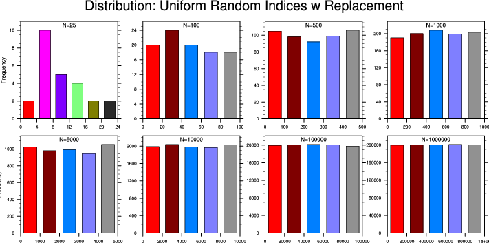
:
These distributions of sampling indices illustrate properties of resampling
with replacement from a uniform distribution using
generate_sample_indices.
Clearly, a reasonably large
N is needed to 'reasonably' sample all combinations.
A simple example of using sampling with replacement to derive a bootstrapped mean
and 95% confidence limits. Here x(N):
   nBoot =   10000
   xBoot = new (nBoot, typeof(x))

   do ns=0,nBoot-1                        ; generate multiple estimates
      iw = generate_sample_indices(N,1)) ; indices with replacement
      xBoot(ns) = dim_avg_n( x(iw), 0 )  ; compute average
   end do

   xAvgBoot = dim_avg_n(xBoot,0)         ; Averages of bootstrapped samples
   xStdBoot = dim_stddev_n(xBoot,0)      ; Std Dev  "        "        "
   xStdErrBoot = xStdBoot/nBoot           ; Std. Error of bootstrapped estimates

   ia = dim_pqsort_n(xBoot, 2, 0)        ; sort bootstrap means into ascending order

   n025     = round(0.025*(nBoot-1),3)    ; indices for sorted array
   n500     = round(0.500*(nBoot-1),3)
   n975     = round(0.975*(nBoot-1),3)

   xBoot_025= xBoot(n025)                 ;  2.5% level
   xBoot_500= xBoot(n500)                 ; 50.0% level  (median)
   xBoot_975= xBoot(n975)                 ; 97.5% level
Note: since 'x(N)' is rank one, the following functions could have been used in place of the
dim_*_n functions: avg, stddev
and qsort. Of course, the arguments would have to change accordingly.
 bootstrap_stat_1.ncl
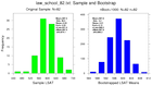
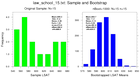
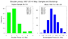
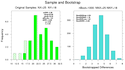
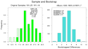
:
These illustrate various properties of the mean (opt@
stat=0)
using different bootstrap sampling parameters.
- use the 82-school data set and resample using the full data set (N=82, n=82)
- use the 82-school data set and resample using 15-member subsets (N=82, n=15)
- use the 15-school data set and resample using only this subset (N=15, n=15)
In all cases, the bootstrapped estimates are generated using
nBoot=1000.
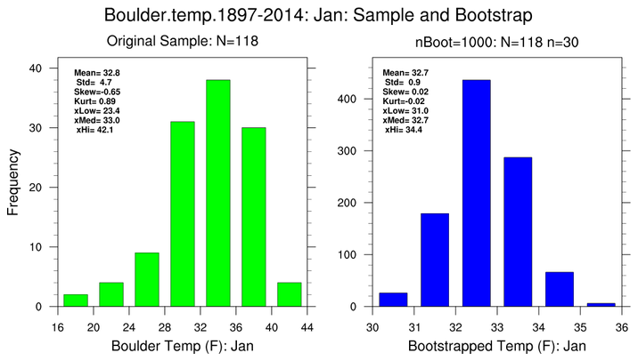
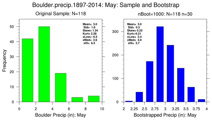
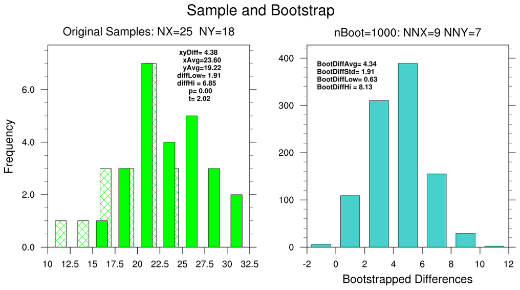
Each figure contains two histograms. The left (green) histogram show the
distribution of the original sample and assorted 'conventional' statistics:
sample mean, standard deviation, standard error, t-value and the 2.5% and 97.5%
confidence bounds . The right (blue) histogram shows the distribution of
bootstrapped sample means; the standard deviation of the bootstrapped means;
the standard error of the bootstrapped means and the 2.5% and 97.5%
bootstrapped values.
 bootstrap_stat_1a.ncl
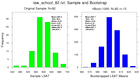
:
This is the same as
bootstrap_stat_1.ncl except the figure includes
graphical markers (here, all asterisks) that indicate the location of the bootstrapped
low (2.5%), median (50%) and high (97.5%) values. The procedure which attaches
the markers to the histogram graphical object is named
histogram_marker.ncl .
 bootstrap_stat_2.ncl
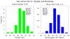
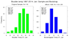
:
Bootstrap January monthly
mean temperatures
(degF; left histogram pair) and May monthly
precipitation totals (inches)
totals (right histogram pair) for Boulder, CO for the period 1897-2014.
Estimate various properties of the mean. The total sample
size for each month is
N=114. Here, 30-year sub-samples (
n=30)
are are generated
nBoot=1000 times.
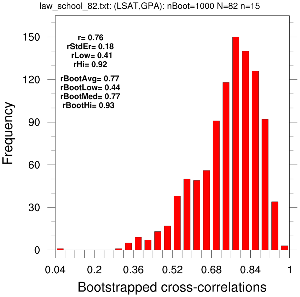
 bootstrap_correl_1.ncl
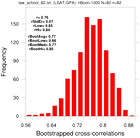
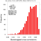
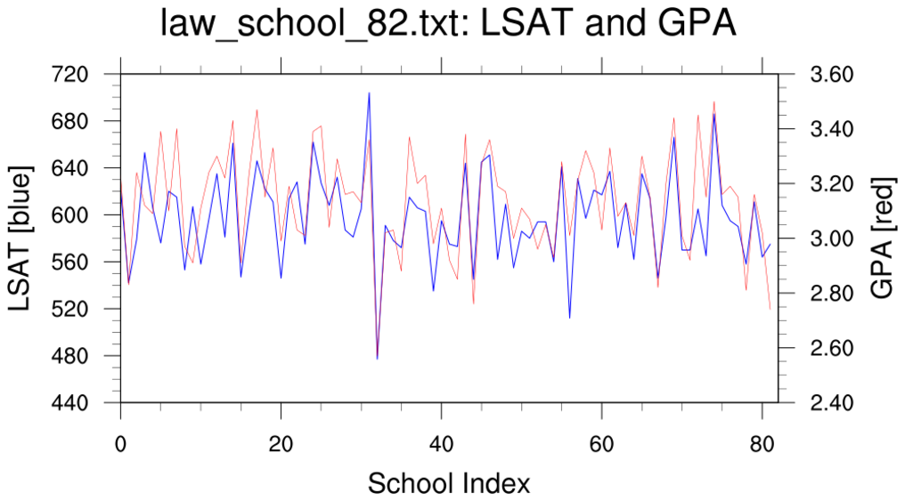
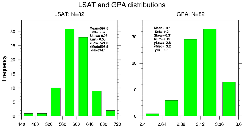
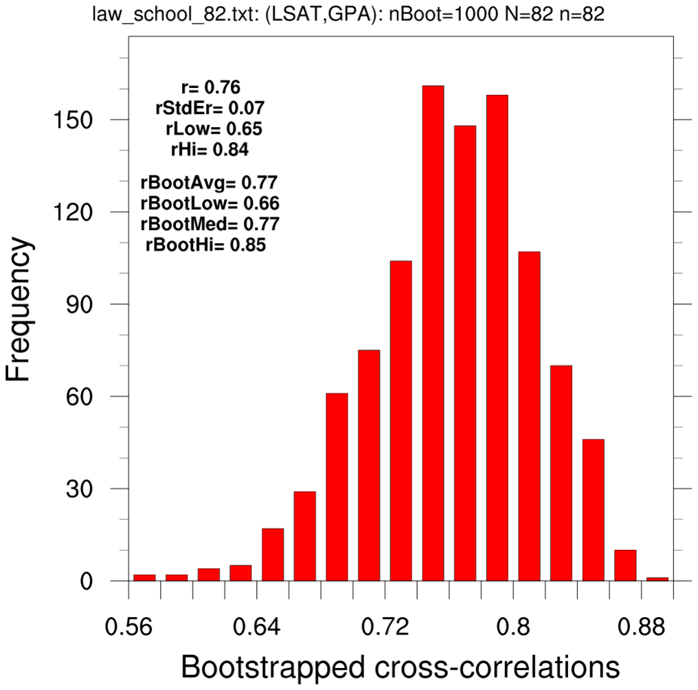
:
These estimate the correlation coefficient between the 82-school LSAT and GPA
using classical statistics and via the bootstrap method.
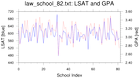
The first rule of data processing is look at your data;
the second rule of data processing is understand your data.
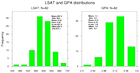
This example illustrates two simple approaches.
- a simple line plot of the 82-school LSAT and GPA values
- histograms of each variable
- use the 82-school data set and resample using the full data set (N=82, n=82)
- use the 82-school data set and resample using 15-member subsets (N=82, n=15)
The two text boxes show values derived using the original single sample the bootstrap estimates. The latter have used the Fischer z-transform to calculate various statistics.
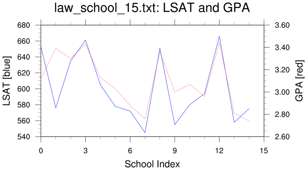
 bootstrap_correl_1.ncl
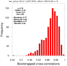
:
This example estimates the correlation coefficient between the 15-school LSAT and GPA
using classical statistics and via the bootstrap method.
This example follows the methodology of the previous example.
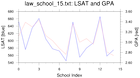
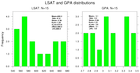
- a simple line plot of the 15-school LSAT and GPA values
- histograms of each variable
- Since N=15, only n=15 is used.
This example (N=15, n=15) 'matches' the Matlab_1 example.
The two text boxes show values derived using the original single sample the bootstrap estimates. The latter have used the Fischer z-transform to calculate various statistics.
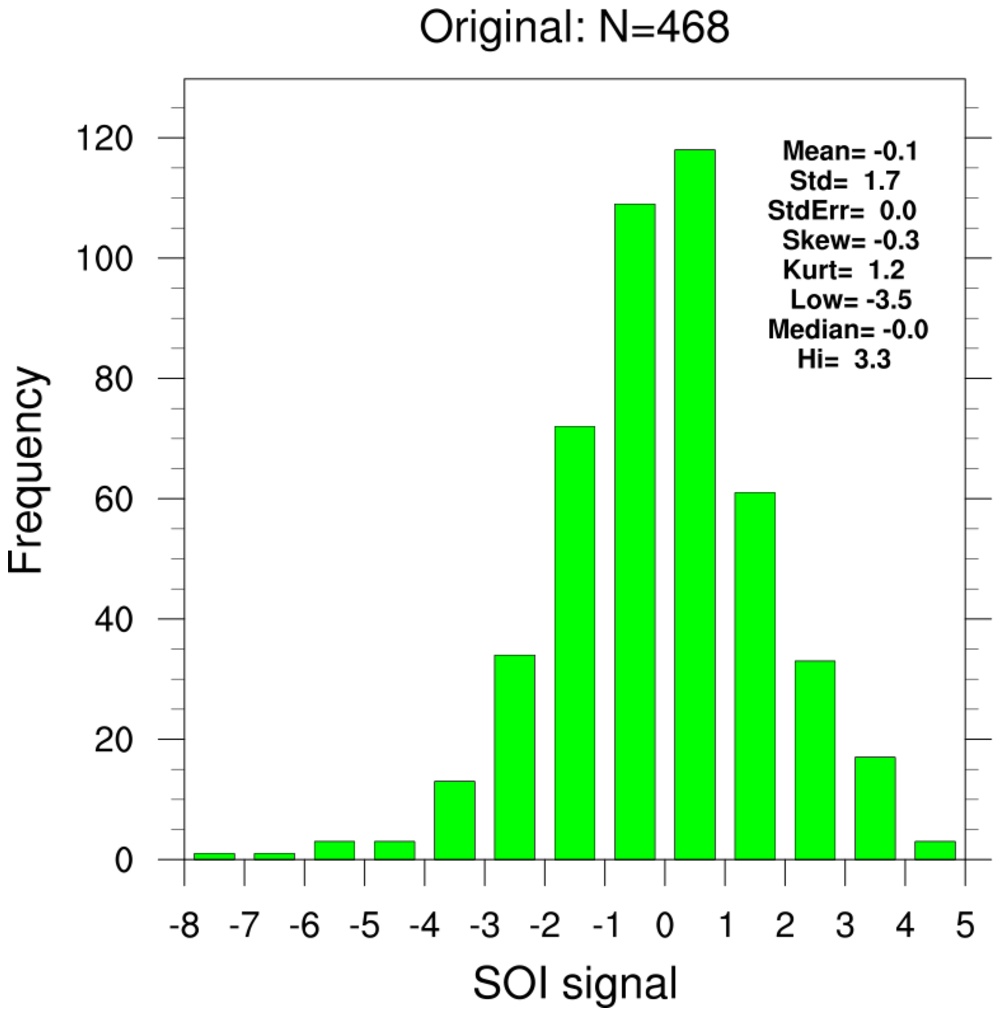
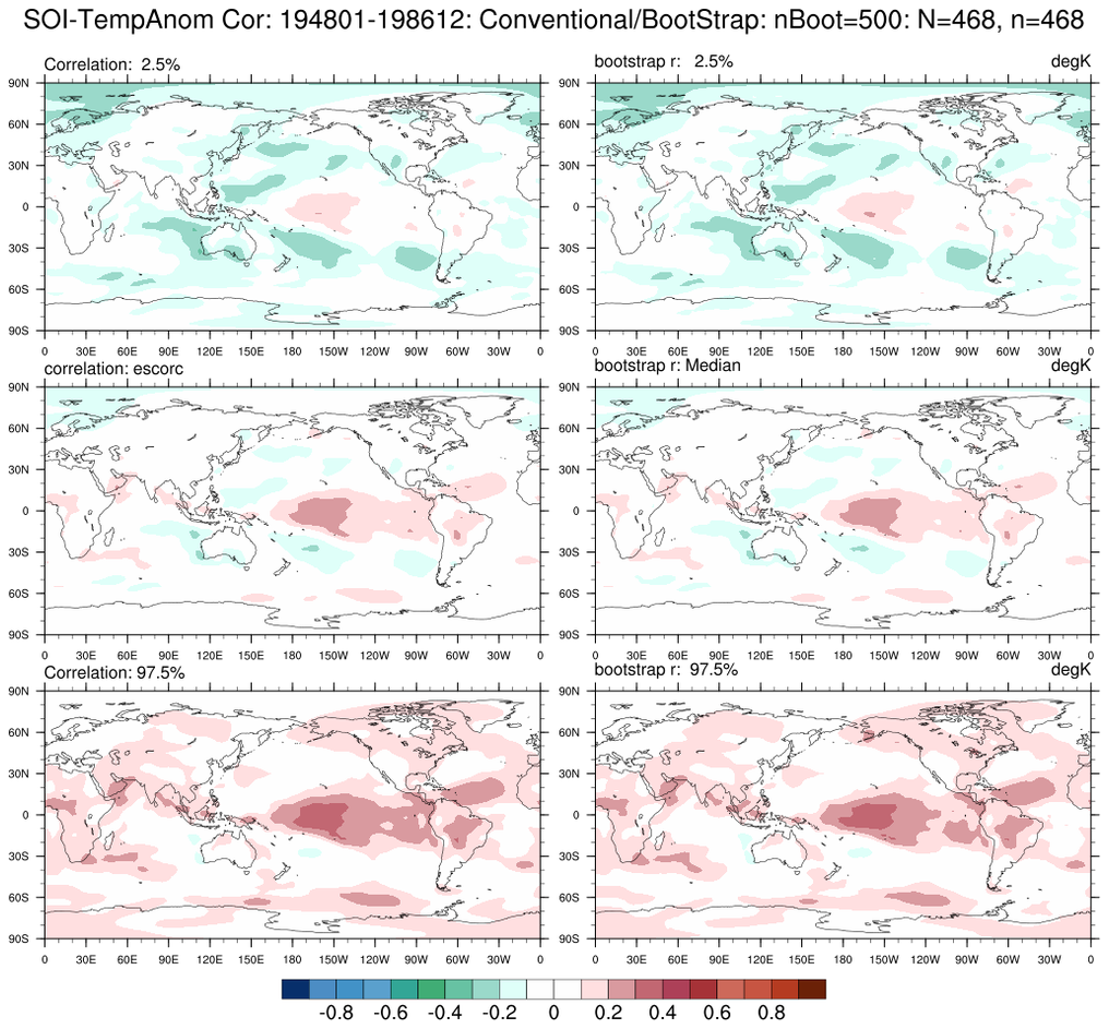
 bootstrap_correl_2.ncl
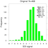
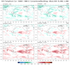
:
Correlate the SOI_SIGNAL (Southern Oscillation Index Signal) and monthly temperature
anomalies. Show the 2.5% and 97.5% limits derived using 'conventional' (left column)
and bootstrap (right column) statistics.
Reference:
Trenberth (1984), "Signal versus Noise in the Southern Oscillation"
Monthly Weather Review 112:326-332
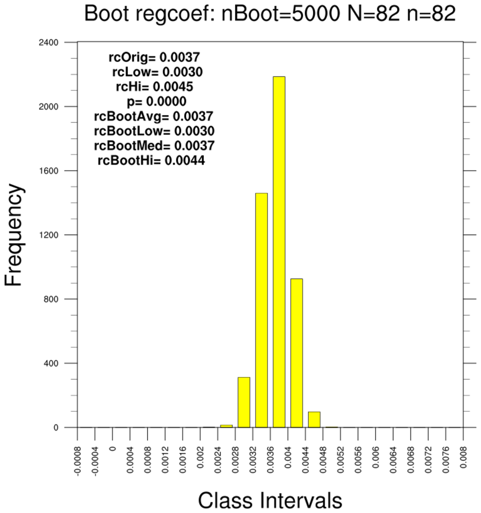
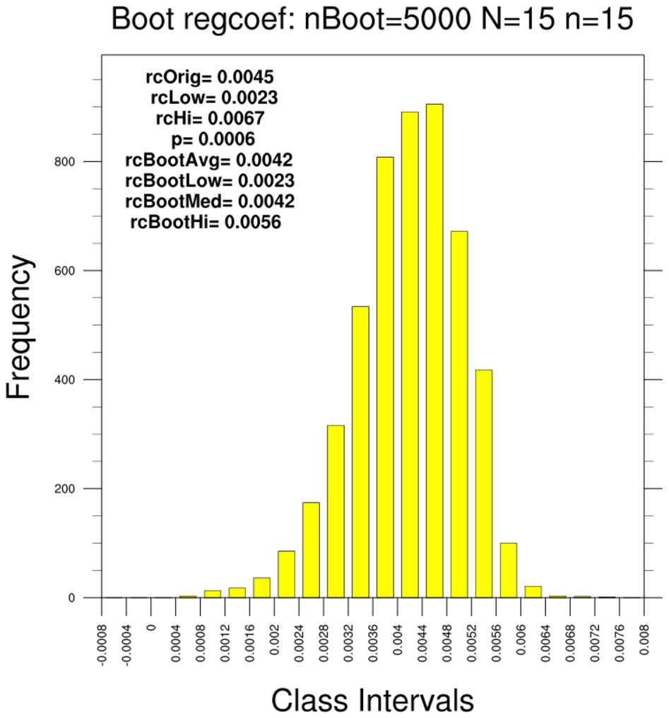
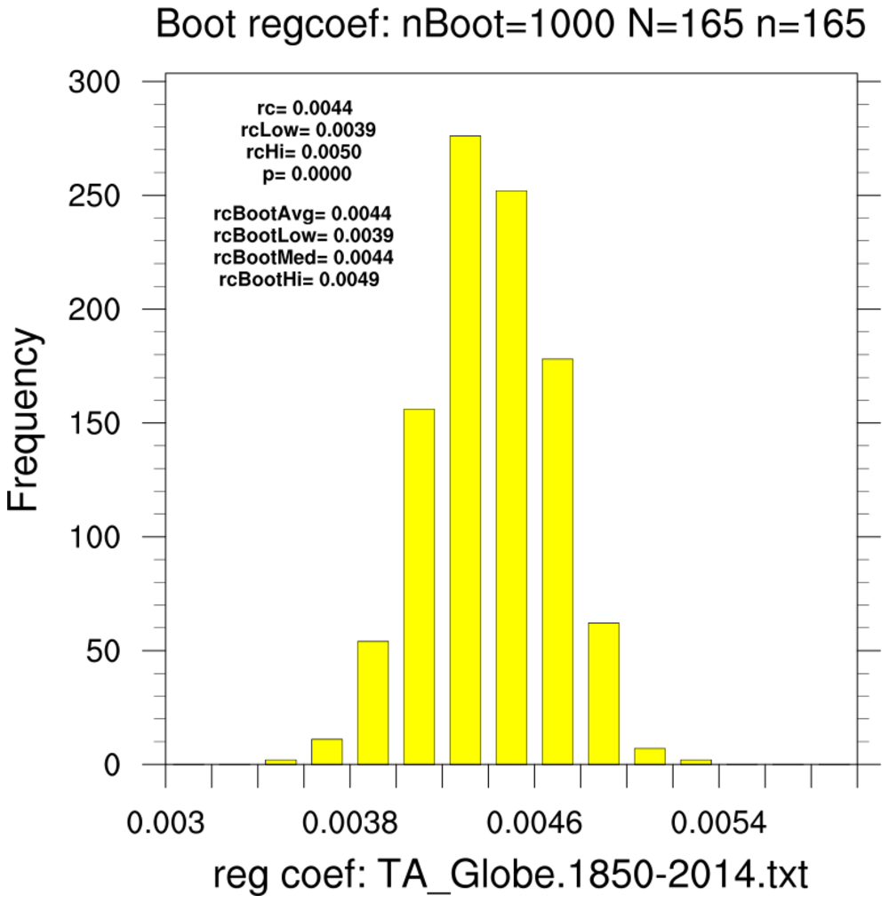
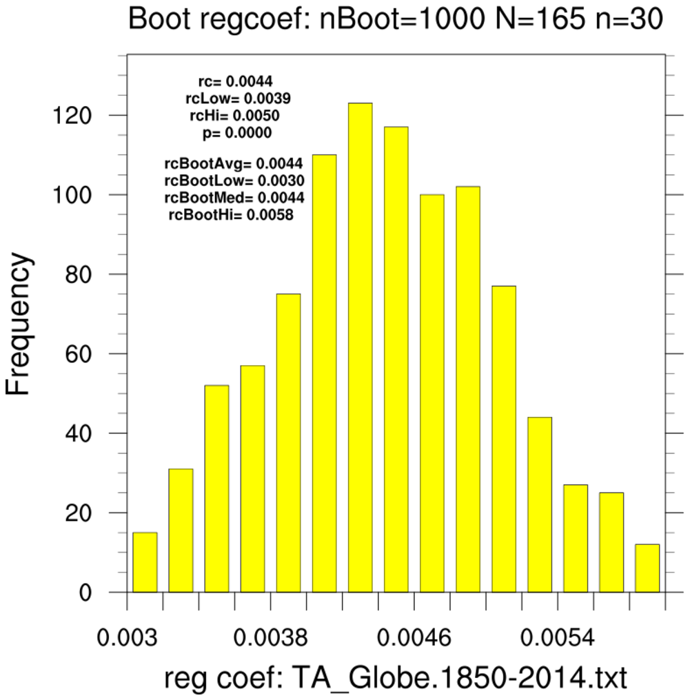
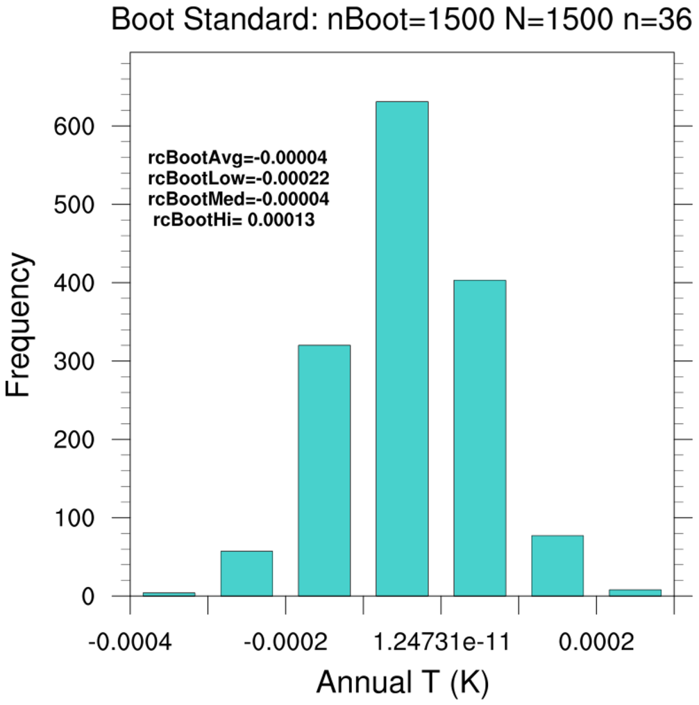
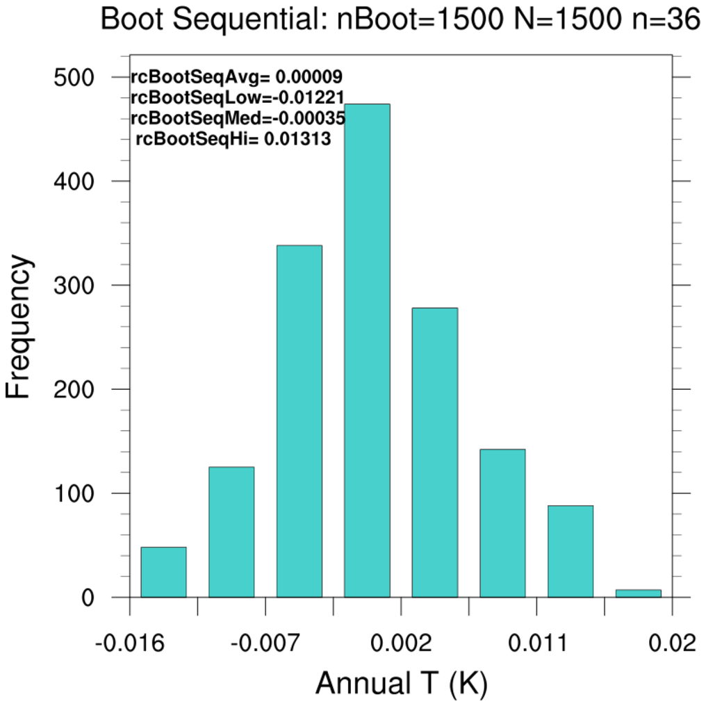
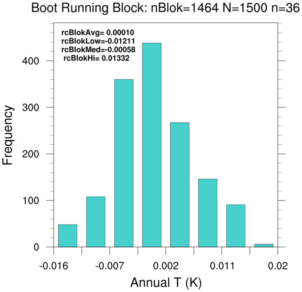
 bootstrap_regcoef_1.ncl
:
These estimate the linear regression coefficient between the LSAT and GPA. Additional
information based upon the original sample is provided via
regline_stats.
- use the 82-school data set and resample using the full data set (N=82, n=82)
- use the 82-school data set and resample using 15-member subsets (N=82, n=15)
- use the 15-school data set and resample using only this subset (N=15, n=15)
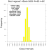
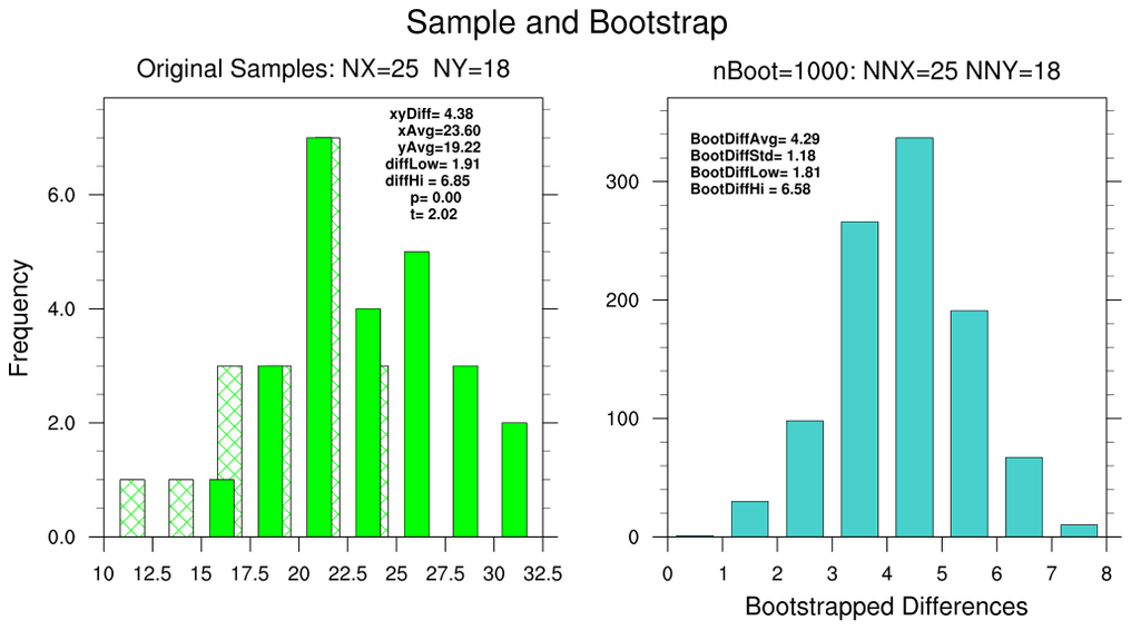
 bootstrap_diff_1.ncl
:
Calculate the conventional and bootstrapped difference statistics between two samples using default
sampling sizes: NX=25 and NY=18. (See the left figure.)
The bootstrapped confidence intervals 'match' the R-generated 95% confidence
values of 2.14 (2.5%) and 6.77 (97.5%). The conventional confidence limits
provided by the reference are 1.96 and 6.80. NCL's and R's p-value=0.0007474 match.
The right figure shows the distribution with user specified sub-sampling:
specifically: opt=True with opt@sample_size_x=9 and opt@sample_size_y=7.
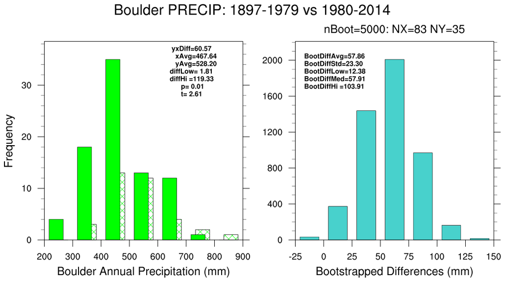
 bootstrap_diff_2.ncl
:
Using Boulder, CO annual precipitation
calculate the conventional and bootstrapped difference statistics between two periods: (a)
1897-1979 and (b) 1980-2014.


