See the eof_n_640.ncl scripts below for examples of using the new xxxx_n functions.
NCL Home>
Application examples>
Data Analysis ||
Data files for some examples

 eof_1.ncl /
eof_1_640.ncl:
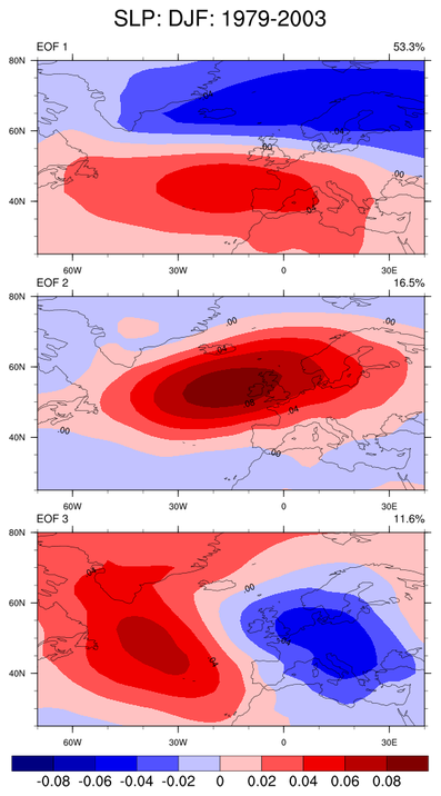
Read sea level pressure;
extract the data spanning 1979-2003; calculate the first three EOFs
over the North Atlantic region for the winter (DJF) season.
The first EOF pattern is commonly identified as the
North Atlantic Oscillation (NAO) mode.
eof_1.ncl /
eof_1_640.ncl:
Read sea level pressure;
extract the data spanning 1979-2003; calculate the first three EOFs
over the North Atlantic region for the winter (DJF) season.
The first EOF pattern is commonly identified as the
North Atlantic Oscillation (NAO) mode.


 mjoclivar_14.ncl:
Example pages containing: tips | resources | functions/procedures
NCL Graphics: EOFs
For historical reasons, NCL contains a suite of EOF functions.
The recommended functions are:
eofunc_n_Wrap,
eofunc_ts_n_Wrap and
eofunc_north.
If no meta data is desired:
eofunc_n and
eofunc_ts_n.
EOF: Standard Empirical Orthogonal Analysis
Standard EOF (aka eigenvector, principal component) analysis yields patterns and time series which are both orthogonal. The derived patterns are a function of the domain and the time period being used. The EOF represntation is optimal in the sense that maximum variance may be accounted for by choosing in order the eigenvectors associated with the largest eigenvalues of the covariance matrix (Kutzback, 1967). However, the EOF procedure is strictly mathematical and is not based upon physics. The results may produce patterns that are similar to physical modes within the the system. However, physical meaning is dependent on your interpretation of the mathematical result.
To be clear, EOF analysis is not a statistical procedure. However, because the results are orthoganal (ie, independent), they have been used as predictor variables in some statistical applications.
Note on signs of EOF analysis (conributed by Andrew Dawson, U. East Anglia)
EOFs are eigenvectors of the covariance matrix formed from the input data. Since an eigenvector can be multiplied by any scalar and still remain an eigenvector, the sign is arbitrary. In a mathematical sense the sign of an eigenvector is rather unimportant. This is why the EOF analysis may yield different signed EOFs for slightly different inputs. Sign only becomes an issue when you wish to interpret the physical meaning (if any) of an eigenvector.
You should approach the interpretation of EOFs by looking at both the EOF pattern and the associated time series together. For example, consider an EOF of sea surface temperature. If your EOF has a positive centre and the associated time series is increasing, then you will interpret this centre as a warming signal. If your EOF had come out the other sign (ie. a negative centre), then the associated time series would also be the opposite sign and you would still interpret the centre as a warming signal.
In essence, the sign flip does not change the physical interpretation of the result. Hence, it is up to you to choose which sign to associate with your EOF patterns for visualisation (remembering that any sign change to an EOF must be applied to the associated time series also). Usually you would simply adjust the sign so that all your EOF patterns with the same physical interpretation also look the same
EEOF: Extended Empirical Orthogonal Analysis
EEOF provides the ability to discern 'common patterns of variability' shared among multiple datasets in both space and time. The "extension" may be in space (S-mode) or in time (T-mode). A visual depiction of these modes is Figure 1 of the Neeti and Eastman (2014) reference. A disadvantage of EEOF "is the possibility that little coherrent persistence exists in the data field so that the functions may obfuscate the spatial coherence identified by traditional technique" (Weare, 1982).
See EEOF examples below.
References:
     A Cautionary Note on the Interpretation of EOFs
     Dietmar, D. and Latif, M.
     J. Climate, 2002:  15: 216-225.

     Empirical eigenvectors of sea-level pressure, surface temperature and precipitation
        complexes over North America
     Kutzbach, J.E.
     Journal of Applied Meteorology (1967): 6, pp. 791-802

     Novel approaches in Extended Principal Component Analysis to compare
        spatio-temporal patterns among multiple image time series
      Neeti, N. and J.R. Eastman
      Remote Sensing of Environment: 148, 25 May 2014, Pages 84-96

     Sampling Errors in the Estimation of Empirical Orthogonal Functions
     North, G. R., T. L. Bell, R. F. Cahalan, and F. J. Moeng
     Mon. Wea. Rev., 1982: 110, 699-706.

     Application of Extended Empirical Orthogonal Function Analysis to
        Interrelationships and Sequential Evolution of Monsoon Fields
     Singh, S,V., R.H. Kriplani
     Mon. Wea. Rev., 1986: 114, 1603-1610.

     Empirical  Orthogonal Function Analysis of Atlantic Ocean Surface Temperatures
     Weare, B.C., R.E. Newell
     Quart. J. Roy. Meteor. Soc., 1977: 103, 467-478.

     Examples of Extended Empirical Orthogonal Function Analyses
      Weare, B.C., J.S. Nasstrom
      Mon. Wea. Review, 1982: 481-485
eof_0.ncl /
eof_0_640.ncl:
These scripts verify the output from eofunc and eofunc_ts
by reading an ascii file containing box data from the book:
   John C Davis
   Satistics and Data Analysis in Geology
   Wiley, 2nd Edition, 1986
   Source Data: page 524 , EOF results: page 537
The results match the book exactly.
The eof_0.ncl and eof_0_640.ncl scripts produce identical results; eof_0_640.ncl uses functions eofunc_n and eofunc_ts_n (added in NCL V6.4.0) to avoid having to reorder the data.
Further illustrated:
- reconstructing the original array from the calculated EOFs and Principal Components (time series)
- computing the sum-of-squares of each EOF to verify that they are normalized
- computing cross correlations of each component to verify there are no cross-component correlations
The source data is available here.
The output from running the above script is here.
eof_0a.ncl:
Same as Eof_0 but here the data are weighted (cosine of latitude). The script illustrates how to 'unweight' the data.
The output from running the above script is here.

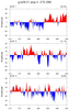
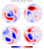
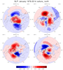
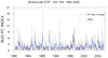
 eof_1.ncl /
eof_1_640.ncl:
Read sea level pressure;
extract the data spanning 1979-2003; calculate the first three EOFs
over the North Atlantic region for the winter (DJF) season.
The first EOF pattern is commonly identified as the
North Atlantic Oscillation (NAO) mode.
eof_1.ncl /
eof_1_640.ncl:
Read sea level pressure;
extract the data spanning 1979-2003; calculate the first three EOFs
over the North Atlantic region for the winter (DJF) season.
The first EOF pattern is commonly identified as the
North Atlantic Oscillation (NAO) mode.
lonFlip is used to rearrange the data to span -180 to 180. Then coordinate subscripting is used to extract the region of interest.
Finally, the resulting principal component time series is normalized by the weights used to get the time series of the mean areal amplitudes.
The eof_0.ncl and eof_0_640.ncl scripts produce identical results; eof_0_640.ncl uses functions eofunc_n and eofunc_ts_n (added in NCL V6.4.0) to avoid having to reorder the data.
The dataset use can be downloaded from:
http://www.esrl.noaa.gov/psd/data/gridded/data.ncep.reanalysis.surface.html
A Python version of eof_1 is available here.
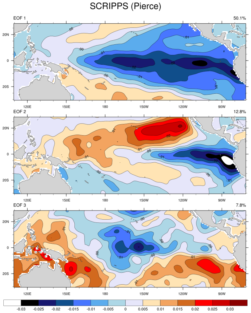
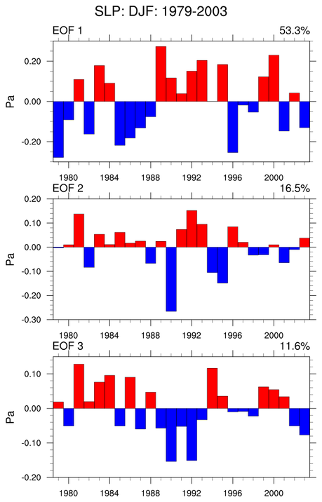
eof_2.ncl eof_2_640.ncl: This is an example posted by David Pierce (Scripps). NCL uses code posted at the the Scripps site. The Scripps example only shows the results from the first EOF. This example shows three patterns and time series. This example was created to illustrate that NCL's eofunc / eofunc_n and eofunc_ts / eofunc_ts_n results match Pierce's. Note that no areal weighting was performed.
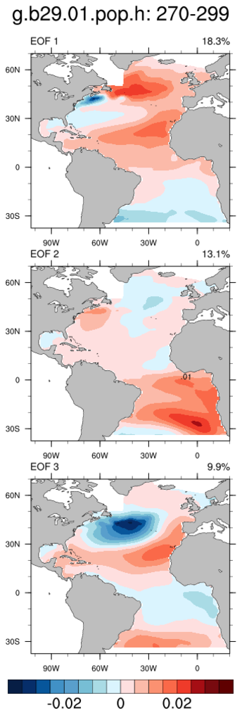
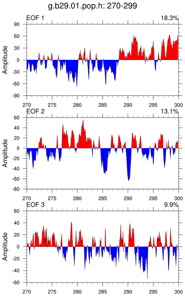
eof_3.ncl / eof_3_640.ncl: From a directory with many POP files, (1) read 30 years spanning years 270-279; (2) compute climatology; (3) compute anomalies; (4) mask out all regions but the Atlantic basin; (5) weight grid by area; (5) compute EOFs; and, (7) plot.
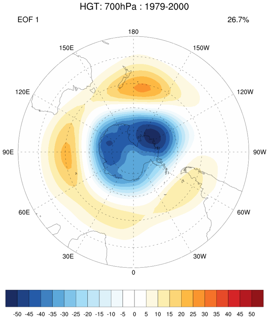

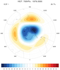
eof_4.ncl / eof_4_640.ncl: Use the approach outlined at the Climate Prediction Center to compute the Antarctic Oscillation (AAO) for the period 1979-2000: Read geopotential height data (source: Reanalysis-2); select 700hPa and data poleward of 20S; compute monthly climatologies and anomalies; weight observations; compute EOFs; normalize the principal components; and project the anomalies via regression.
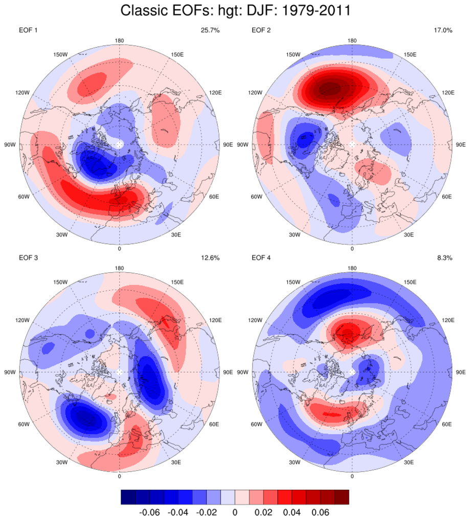
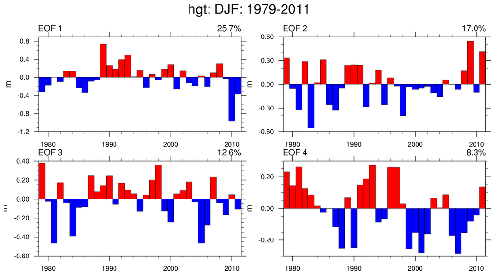

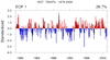
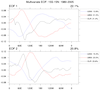
eof_5.ncl / eof_5_640.ncl: Compute EOFs for the northern hemisphere height field at 500hPa. Use cd_calendar to create an array containing time in the form of YYYYMM. Then use ind to determine the index values corresponding data from 1979-2011. Read the desired data using NCL's coordinate subscripting. Compute standard EOFs via eofunc_Wrap and the corresponding time series via eofunc_ts_Wrap. Because we want to do a varimax rotation 6 EOFs were computed. This (neof=6) is arbitrary but it should be large enough to allow eofunc_varimax_Wrap to reorthogonalize the subset. Finally, eofunc_varimax_reorder is used to place the output into descending order. The attribute pcvar_varimax represents the variance explained after the varimax rotation has been applied.

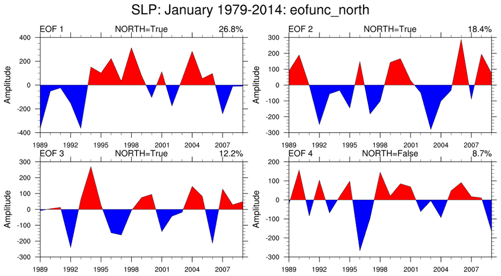
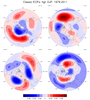
eof_6.ncl / eof_6_640.ncl: Compute EOFs for the northern hemisphere January sea level pressures from 1989-2009. The eofunc_north is used to assess if eigenvalues are distinct.
if the prinfo argument is set to True. The following will be printed.
          dlam      low      pcvar     high    sig
(0)	8.28161   18.5539   26.8355   35.1171  True
(1)	5.68727   12.7416   18.4289   24.1161  True
(2)	3.76075   8.42548   12.1862   15.947   True
(3)	2.67866   6.00119   8.67985   11.3585  False
where 'dlam' is the 'shift' (North's term).
EEOF: Extended Empirical Orthogonal Analysis Examples
Shikha Singh (Scientist, Indian Institute of Tropical Meteorology, Pune, India) has suggested multiple methods for combining different variables with common dimensionality: (time,lat,lon).
For simplicity, two variables (var1, var2) with dimensionality (ntim,nlat,mlon) are used to illustrate the T-mode approach. Generally for climate, it is assumed that the variables contain anomalies from the mean annual cycle. Because the anomaly variables may have different variances, normalized values should be input to the function. Specifically:
  var1 = ...anomalies...
  var2 = ...anomalies...

  dimv = dimsizes(var1)
  ntim = dimv(0)
  nlat = dimv(1)
  mlon = dimv(2)

  std1 = dim_stddev_n(var1,0)  ; local (grid point, station)  standard deviations
  std2 = dim_stddev_n(var2,0)
or
  std1 = stddev(var1)           ; overall (field) standard deviation
  std2 = stddev(var2)

  nvar = 2
                    ; T-mode
                    ; 0  ,  1  ,  2  ,  3   ;  dimension numbers
  new_data = new((/nvar, ntim, nlat, mlon/), typeof(var1),getFillValue(var1))
  new_data(0,:,:,:) =  var1/std1
  new_data(1,:,:,:) =  var2/std2

  NEW_DATA = reshape(new_data,(/2*ntim,nlat,mlon/))
  printVarSummary(NEW_DATA)

  neof = 3          ; # of desired EOFs
  ndim = 1          ; dimension number for 'time'
  eeof = eofunc_n(NEW_DATA, neof, False, ndim)
  printVarSummary(eeof)
Dr. Singh also suggested the following for S-mode EEOF using longitude and latitude spatial extensions.
  ; Joining the data along the longitude axis

  new_data1 = new((/2*mlon, nlat, time/),typeof(var1),getFillValue(var1))
  new_data1(0:mlon-1,:,:)       = var1
  new_data1(mlon:2*mlon-1,:,:)  = var2

  ; Joining the data along latitude axis
  new_data2 =new((/mlon, 2*nlat, time/), typeof(var1),typeof(var1),getFillValue(var1))
  new_data2(:,0:nlat-1,:,:)     = var1
  new_data2(:,nlat:2*nlat-1,:,:)= var2
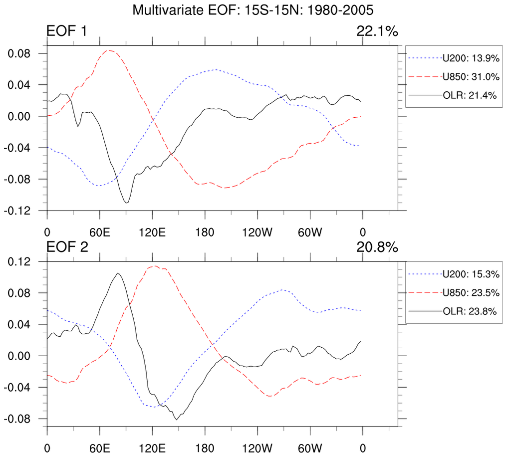
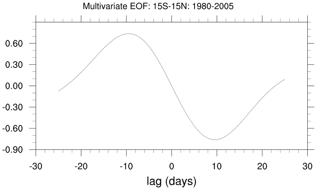
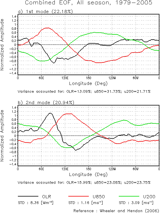
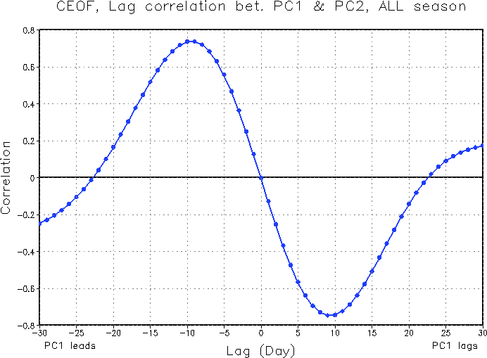
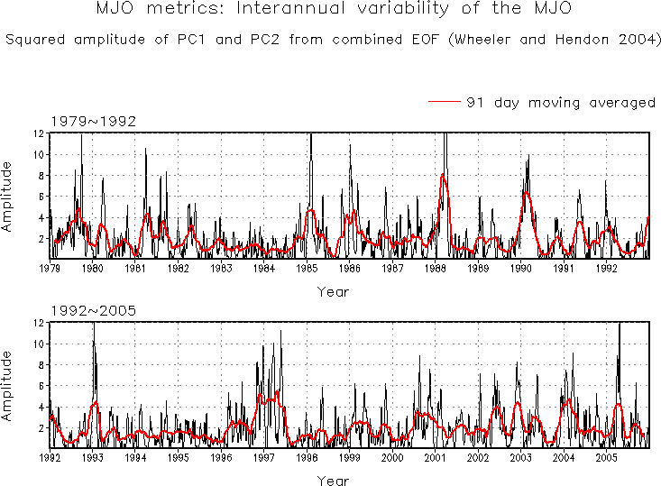
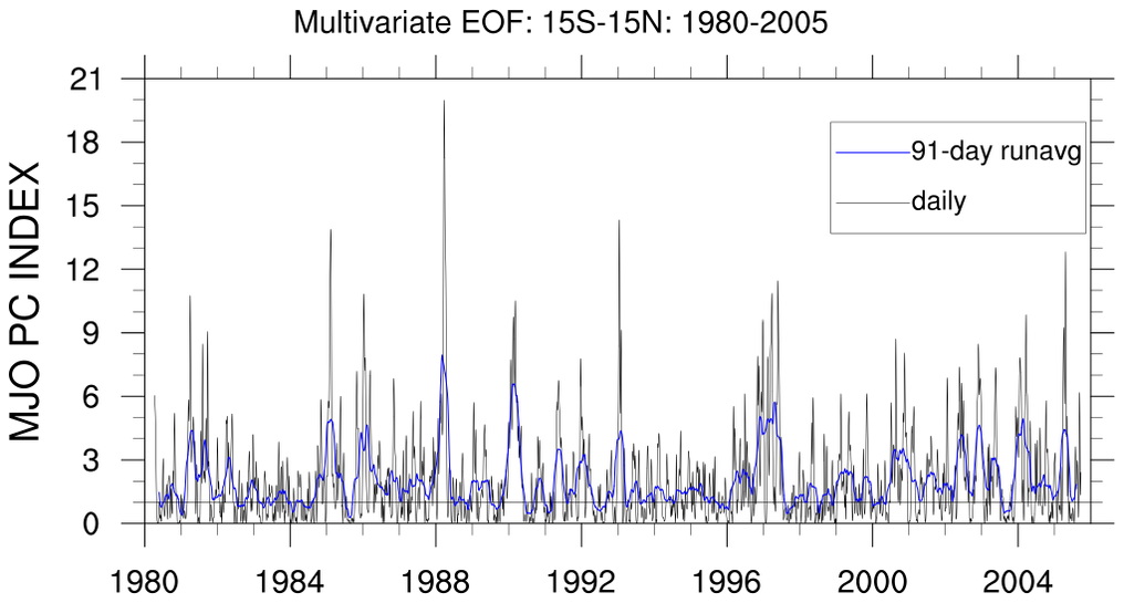 mjoclivar_14.ncl:
The data from OLR, Uwind, Vwind are averaged along latitude to make 2D data. The 3 variables are then combined into a bigger matrix: (time,space).
Multivariate (Combined) EOF; cross-correlations between EOF1 and EOF2; time-series of (PC1^2 + PC2^2) and 91-day running mean.
This script was updated 2 March 2015. Marcus N. Morgan (Florida Institute of Technology) submitted the code segment that calculates the percent variance for each component in the multivariate EOF.
This script was updated 29 July 2016. Eun-Pa Lim: Bureau of Meteorology, Australis
For comparison, the equivalent 3 plots from the Korean MJO-Diagnostics are (a) eof_all; (b) lag_all (c) time series