NCL Home>
Application examples>
Plot techniques ||
Data files for some examples
Example pages containing:
tips |
resources |
functions/procedures
NCL Graphics: Masking
Masking refers to the technique of not drawing certain portions of
your data over areas you are not interested in.
Various ways to do masking include:
- using the mask function to change certain
values in your data to missing,
- using gc_inout to change certain
values in your data to missing,
- using graphical resources to control masking,
- changing the drawing order of certain plot elements to control
what gets drawn when.
You may also want to see the draw order
applications page to see examples of controlling graphical masking
by changing the draw order of certain plot elements.
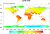
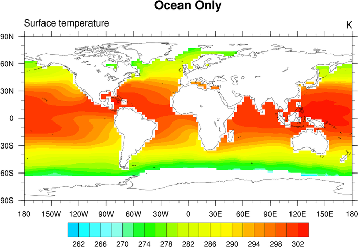
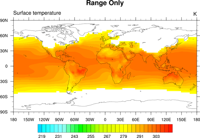
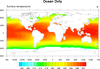 mask_1.ncl
: Demonstrates the use of
the
mask
function and a masking array to mask out land or ocean.
The NCL mask
function can be a bit confusing. It sets all values to missing that DO
NOT equal the mask array. To mask out the ocean, you put in the land
value and vice versa.
A Python version of this projection is available here.
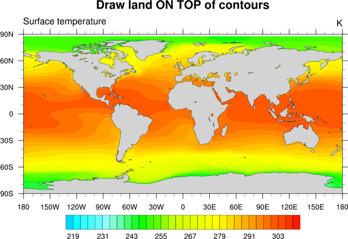
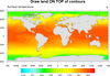 mask_2.ncl
: Uses resources to draw
land on top of the contours.
cnFillDrawOrder = "Predraw"
draws the contours first. If necessary, you can also specify that the
contour lines be drawn first as well by setting cnLineDrawOrder = "Predraw".
A Python version of this projection is available here.
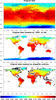
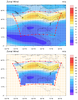
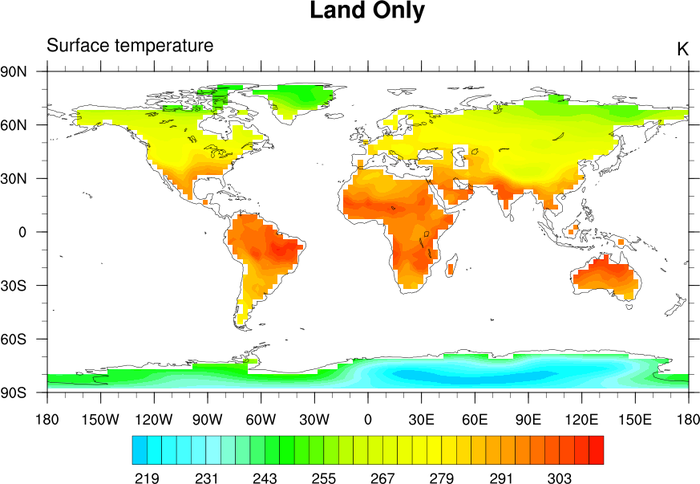
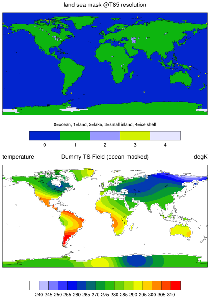
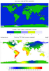 mask_5.ncl
: The shea_util function
landsea_mask
can be used to create a landsea mask when one is not available for your particular dataset. This example demonstrates
how to use
landsea_mask to calculate a mask based on a particular resolution (in
this case t85), and how to apply that mask to mask out all the ocean points from the data array.
The top plot shows the calculated T85 land sea mask. Note that at this resolution some islands (notably Hawaii) are not labeled as
land or as small islands. This can be due to a variety of reasons, including the resolution of the data, the resolution of
the 1x1 basemap, or whether the centers of the grid boxes are over the islands themselves. Note that the file that is
returned by landsea_mask can be easily modified, as can the basemap that is downloadable
off of the landsea_mask documentation page.
The bottom plot shows a surface temperature field at T85 resolution that has had the ocean points masked out by using the land sea
mask shown in the top plot.
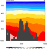
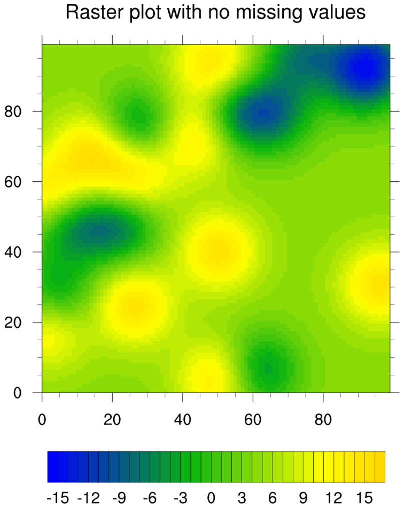
 mask_7.ncl
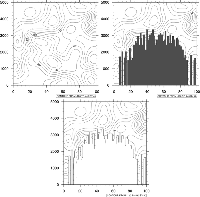
: This example shows how to
mask out areas of a contour plot that are below a certain threshold, in this case topography.
The first frame shows the unmasked data array.
The second frame shows the data array masked by the topography, with the missing areas
filled via cnMissingValFillColor. Note that to use cnMissingValFillColor, one also has to set cnFillOn to True. As we
do not wish to color fill the contour field in this case, we simply set cnFillColor to the background
color (white in this case).
The third frame shows the data array masked by the topography, with the missing areas outlined. cnMissingValPerimOn needs to be set to True to outline the missing areas.

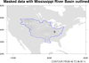
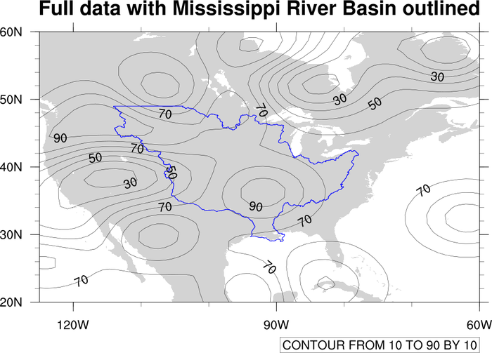
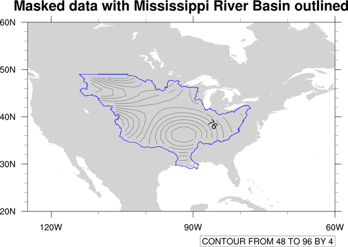
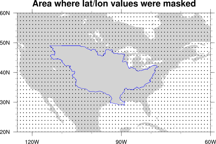
 mask_9.ncl
: Demonstrates
using
gc_inout to mask an area in your
data array using a geographical outline.
This particular example reads
a shapefile to get an outline of the
Mississippi River Basin. You then have the option of masking out all
areas inside or outside this outline.
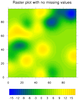

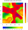 mask_10.ncl
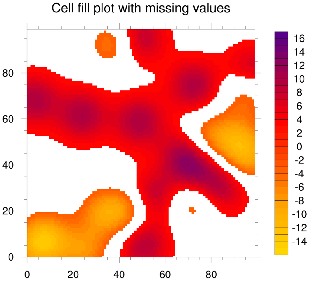
: Demonstrates how to
overlay a cell fill plot on a raster plot, filling the missing value
areas of the cell fill plot with transparency so you can see the first
contour plot underneath.
The cnMissingValFillColor resource
is set to -1 to get the transparency. You have to use a
cnFillMode of "CellFill" for the
second plot, because transparency isn't available for
"RasterFill". ("AreaFill", the default, would also work.)
 mask_11.ncl
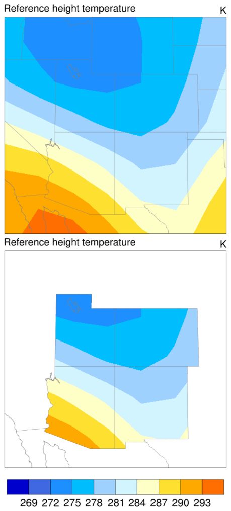
: Similar to
example 8,
this script shows how to show a color filled contour field only over those areas
specified in
mpFillAreaSpecifiers.
In this example the Earth..4
database is used by setting the mpDataSetName resource. This database
has many areas, and all can be specified in mpFillAreaSpecifiers. Note that under the
Area Name column in the table on the Earth..4 page there
are a number of words bolded. The bolded part of the area name is unique, and can be used to specify a specific area.
The following areas were specified: (/"Arizona","New Mexico","Conterminous US: Utah",
"Conterminous US: Colorado", "Great Salt Lake"/). The reason "Conterminous US" was needed
before Colorado and Utah is because there are other areas in the Earth..4
database named Utah and Colorado, namely Utah county in Utah and Colorado county in Texas. As these areas are being specified in
mpOutlineSpecifiers and mpFillAreaSpecifiers, these areas would
also be outlined and filled if "Conterminous US" was not present. The reason Great Salt Lake was specified is because
all inland water areas were being map color filled white, and by specifying Great Salt Lake in
mpOutlineSpecifiers and mpFillAreaSpecifiers NCL will not
color fill the lake white.
 mask_12.ncl
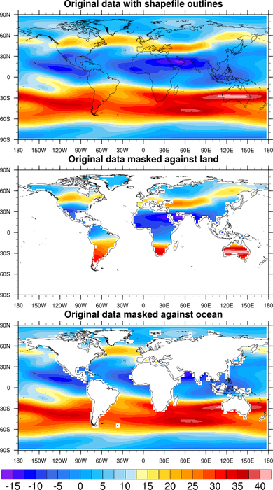
: This example shows how
to use a shapefile that contains polygon outlines to create a data
mask for a variable with 1D coordinate arrays. The mask array is then
written to a copy of the input file.
In this case, the shapefile contains coastal outlines, which a land
mask is created from. See the function "create_mask_from_shapefile"
in the "mask_12.ncl" script. This function only works for data that
contains coordinate arrays. You will need to modify it to work with
curvilinear or unstructured data.
You should be able to use any shapefile that contains polygon data
(point and polyline data won't work) to create the desired mask.
The shapefile used in this example was part of a compressed file,
"GSHHS_shp_2.2.0.zip", downloaded from:
http://www.ngdc.noaa.gov/mgg/shorelines/data/gshhs/oldversions/version2.2.0/
You need to uncompress it with the "unzip" command. You can use any
of the other shapefiles that are included with this file, but they are
potentially a higher resolution, and hence creating the mask will take
longer.
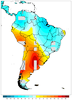
 mask_13.ncl
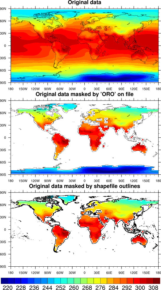
: This example
uses the same "create_mask_from_shapefile" function as the
previous example, to compare the mask with the "ORO" mask
already on the file (same data used in example mask_1.ncl).
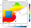
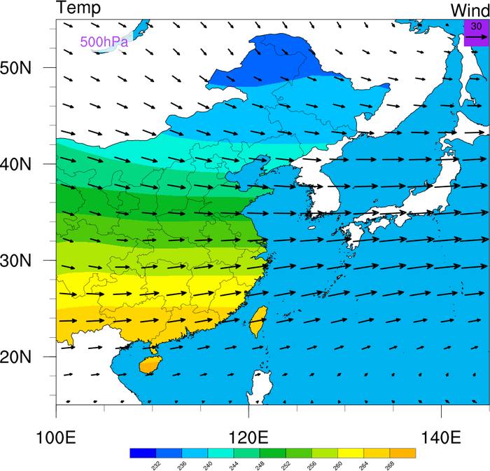
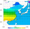 overlay_11.ncl
:
This example shows how to overlay vectors on top of a filled contour plot,
where the contours are masked by a geographical area and the vectors
are not. The masking is accomplished by setting:
  mpres@mpDataBaseVersion   = "MediumRes"
  mpres@mpMaskAreaSpecifiers = (/"China:states","Taiwan"/)
The mask area specifier names are part of the
predefined group
names available in the "MediumRes" map database.
This script was written by Yang Zhao (CAMS) (Chinese Academy of
Meteorological Sciences).
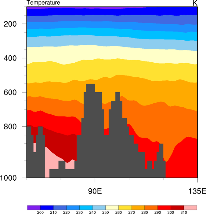
 mask_14.ncl
: This example
shows how to mask data based on terrain data read from a separate
file. The terrain data is regridded to the data to be masked
using
area_hi2lores_Wrap.
This script was written by Yang Zhao (CAMS) (Chinese Academy of
Meteorological Sciences).
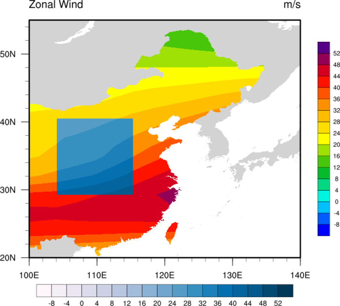
 mask_15.ncl
: This example
shows how to draw two filled contour plots on top of one
another. The top plot has a rectangular "hole" of missing
data, allowing you to see part of the base plot underneath.
The original version of this script was written by Yang Zhao and
Yuhong Wang (CAMS) (Chinese Academy of Meteorological Sciences).
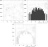
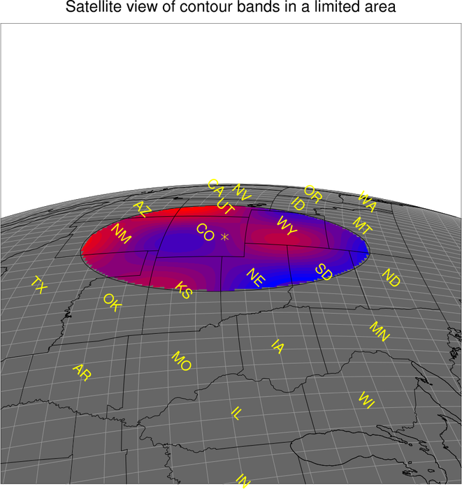
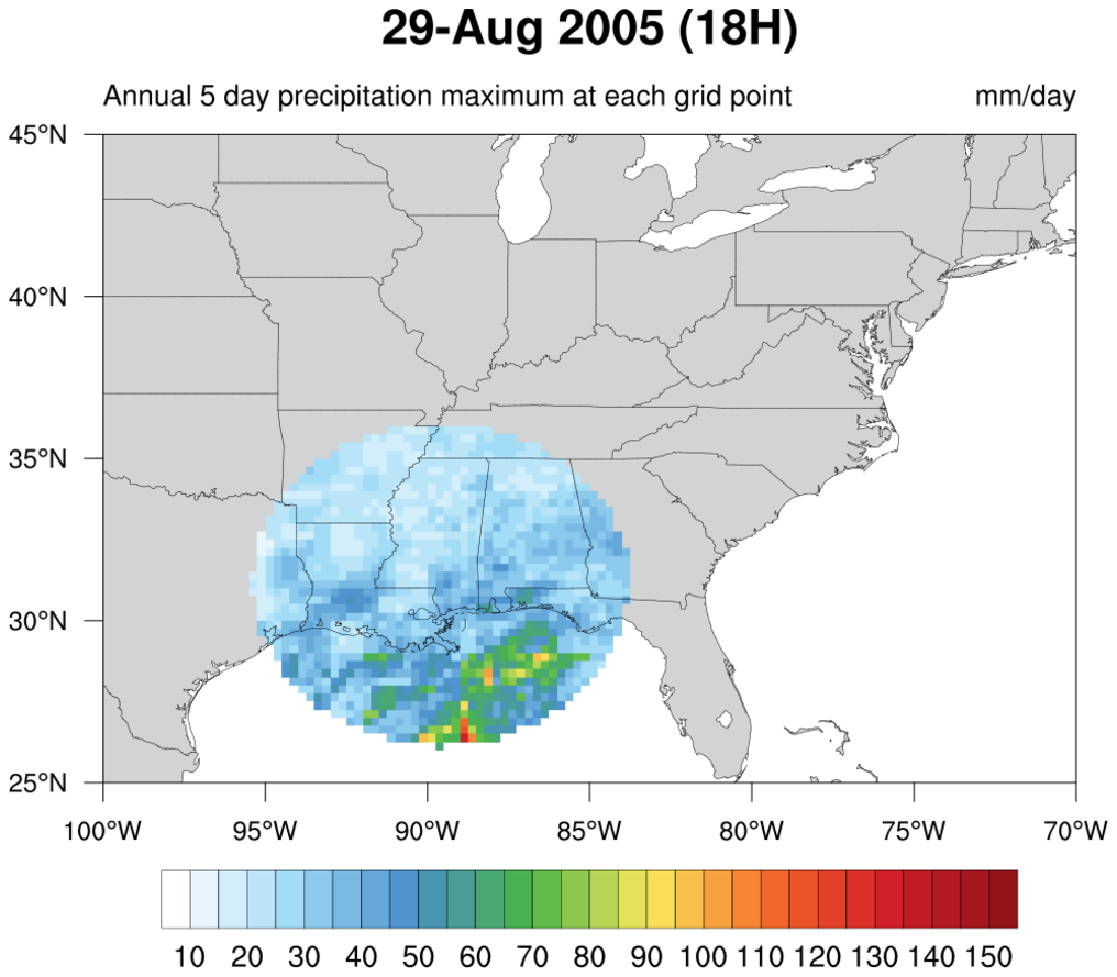
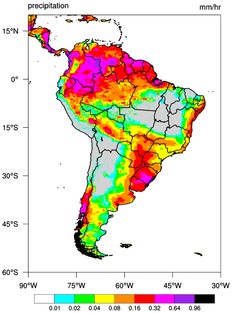
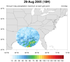 Katrina_circle.ncl
:
This script plots the 5-day running average of precipitation for an
entire year (2005). It shows a unique way of displaying filled
contours in a circle, by using
nggcog in conjunction
with
gc_inout to mask data inside a great circle.
See the Unique examples page
for another version of this script that generates a histogram of the values,
and for an animation of both scripts.
This code was contributed by Jake Huff, a Masters student in the
Climate Extremes Modeling Group at Stony Brook University.
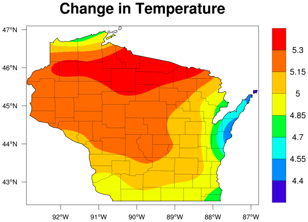
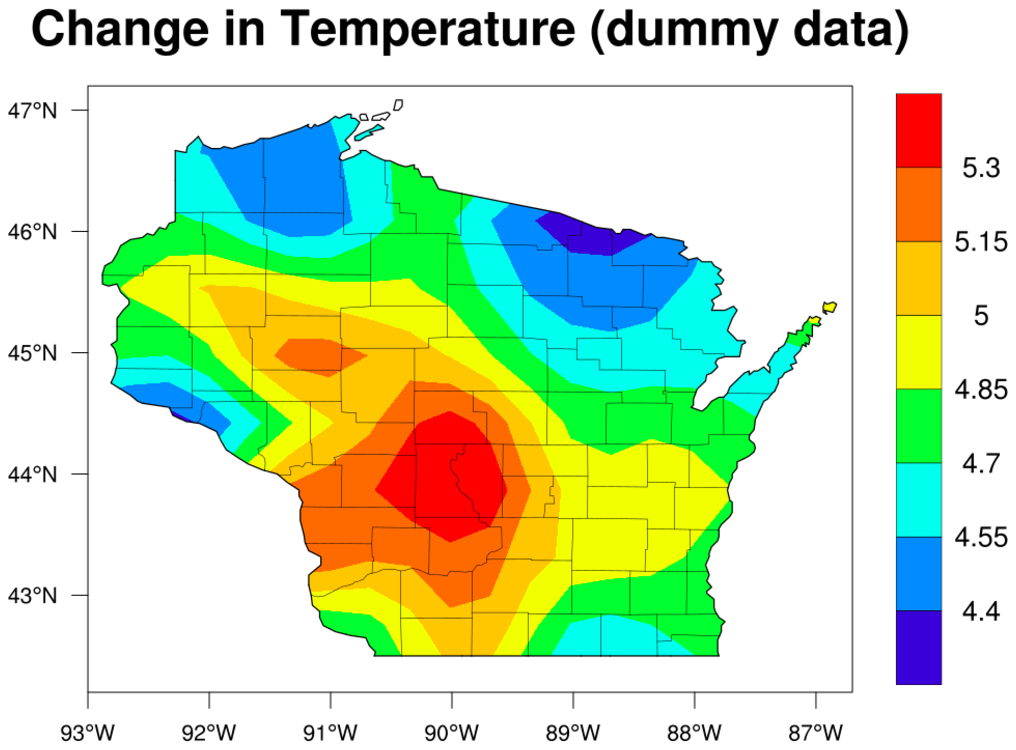
 mask_16.ncl
 /
mask_annotate_16.ncl:
This example, which uses dummy data, shows how to draw filled contours over gray land,
with the ocean filled in white to mask out the filled contours over ocean.
The dummy data was generated using
generate_2d_array, with
random missing values added for illustrative purposes. For an example using real data
see examples mask_17.ncl / mask_annotate_17.ncl below.
In order to draw filled land, followed by filled contours, followed
by filled ocean, you have to create two plots.
The mask_16.ncl script creates and draws the contour/map plot twice:
the first time with filled contours drawn over gray land and
transparent ocean (the ocean color is arbitrary), and second time with
the ocean filled in white, the land transparent, and the filled
contours also transparent so you don't end up with filled contours
over ocean again.
The mask_annotate_16.ncl script creates a contour/map plot with filled contours
over gray land and transparent ocean and a map only plot of the exact same size
with white ocean and transparent land. You then have two choices for drawing the two plots:
you can simply draw both of them, or you can add one as an annotation of the other using
gsn_add_annotation. Both methods are shown in this script,
and they both produce the same image. The annotation method is generally the preferred method,
because this will allow you to panel a series of these plots later with
gsn_panel.
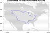
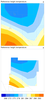
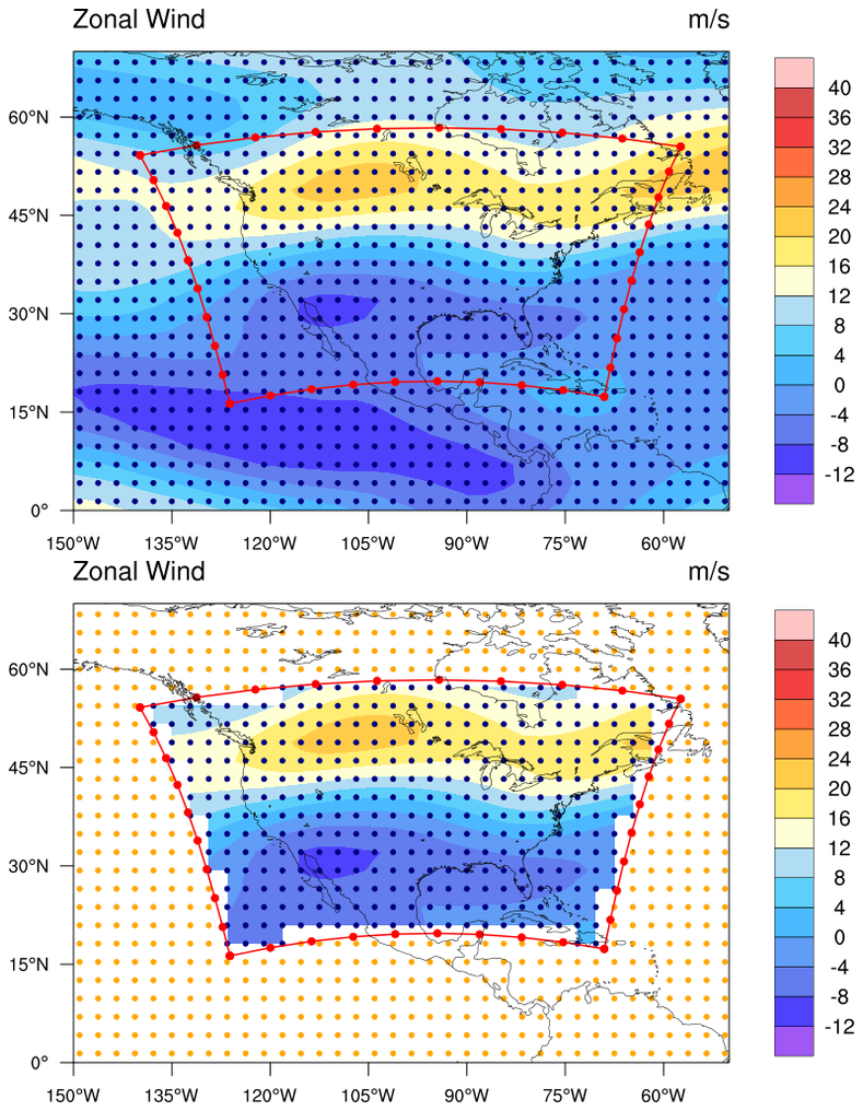
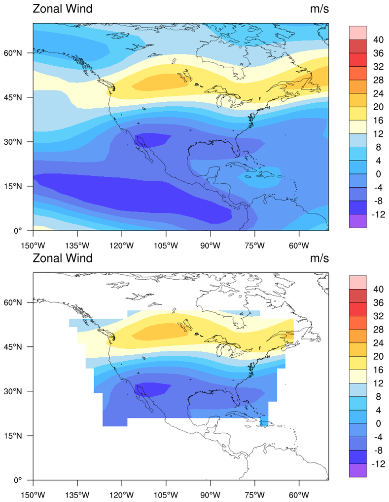
 mask_18.ncl
: This example
shows how to create a lat/lon polygon from the boundary of a lambert
conformal plot, and then use this polygon to mask data with
gc_inout. See the "get_latlon_bounding_polygon"
and "create_mask_array" functions.
The data being masked is a simple 2D array which has coordinate
arrays. If you need to mask data that is not rectilinear, then you'll
need to modify the "create_mask_array" function and change lat1d/lon1d
to represent your lat/lon grid or mesh.
Both images contain the original data in the top plot, and the masked
data in the bottom plot. The first image has primitives added (markers
and lines) to show the location of the lambert conformal boundary, and
the location of the missing and non-missing data.

