NCL Home>
Application examples>
Data Analysis ||
Data files for some examples
Example pages containing:
tips |
resources |
functions/procedures
NCL: Regression & Trend
Regression:There are four primary regression functions:
- (a) regline which performs simple linear regression; y(:)~r*x(:)+y0;
- (b) regline_stats which performs linear regression
and, additionally, returns confidence estimates and an ANOVA table.
- (c) regCoef which performs simple linear regression on multi-dimensional arrays
- (d) reg_multlin_stats which performs
multiple linear regression (v6.2.0) and , additionally,
returns confidence estimates and an ANOVA table.
There are two other regression functions (regcoef,
reg_multlin) but these are used less frequently. They
are maintained for backward compatibility only.
Linear and multiple linear regression models make a number of
assumptions
about the independent predictor variable(s) and the dependent response variable (predictand).
A primary assumption is that the response variable is a linear combination
of the regression coefficients and the predictor variables. Further, the
predictor variable(s) are assumed to be uncorrelated.
Trend: In addition to regression, other methods can be used to assess trend.
The well known
Mann-Kendall non-parametric trend test statistically assesses if there is a monotonic upward or downward trend
over some time period. A monotonic upward (downward) trend means that the variable consistently increases (decreases) through time, but the trend may or may not be linear. The MK test can be used in place of a parametric linear regression analysis, which can be used to test if the slope of the estimated linear regression line is different from zero. The regression analysis requires that the residuals from the fitted regression line be normally distributed; an assumption not required by the MK test, that is, the MK test is a non-parametric (distribution-free) test.
The Theil-Sen trend estimation method "is insensitive to outliers; it can be significantly more accurate than simple linear regression for skewed and heteroskedastic data, and competes well against non-robust least squares even for normally distributed data in terms of statistical power. It has been called 'the most popular nonparametric technique for estimating a linear trend'."
The trend_manken function performs both the Mann-Kendall test and Theil-Sen trend estimation.
The USA's Environmental Agency provides a basic description of use and interpretation:
Statistical Analysis for Monotonic Trends.
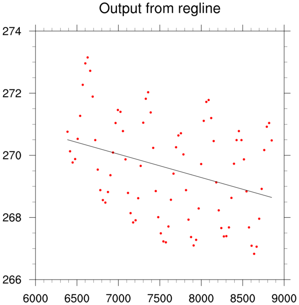
 regress_1.ncl
:
Tabular data (
regress_1.txt )
contained within an ascii file are read. The
regline function is used to calculate
the least squared regression line for a one dimensional array.
Here, the regression coefficient is synonymous with the slope or trend.
     Variable: rc

     Number Of Attributes: 7
       yintercept :	275.3205350166454
       yave :	269.5734479950696
       xave :	7618.59756097561
       nptxy :	82
       rstd :	0.000234703
       tval :	-3.21405918

     (0)	-0.000754349
A Python version of this projection is available here.

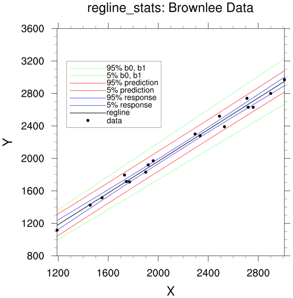
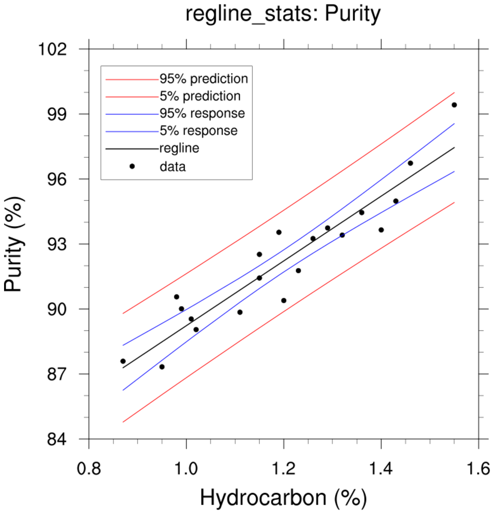
 regress_1a.ncl
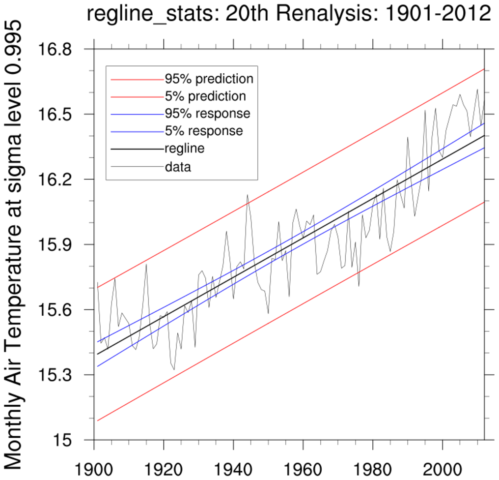
:
See
regline_stats Example 1. This uses the information
provided in the
NCL 6.4.0 release to plot 95% mean response (blue), prediction limits (red) and
lines derived using the 95% limits if the slope and y-intercept (green).
       Variable: rc
        Type: float
        Total Size: 4 bytes
                    1 values
        Number of Dimensions: 1
        Dimensions and sizes:   [1]
        Coordinates:
        Number Of Attributes: 38
          _FillValue :  9.96921e+36

          long_name :   simple linear regression
          model :       Yest = b(0) + b(1)*X

          N :   18                              ; # of observations
          NP :  1                               ; # of predictor variables
          M :   2                               ; # of returned coefficients
          bstd :        (  0, 0.9947125 )       ; standardized regression coefficient
                                                ; [ignore 1st element]

                                                ; ANOVA information: SS=>Sum of Squares
          SST : 4823324                         ; Total SS:      sum((Y-Yavg)^2)
          SSE : 50871.91                        ; Residual SS:   sum((Yest-Y)^2)
          SSR : 4772452                         ; sum((Yest-Yavg)^2)

          MST : 283724.9
          MSE : 3179.494
          MSE_dof :     16
          MSR : 4772452

          RSE : 56.387                          ; residual standard error; sqrt(MSE)
          RSE_dof :     15

          F :   1501.01                         ; MSR/MSE
          F_dof :       ( 1, 16 )
          F_pval :      1.51066e-17

          r2 :  0.989453            ; square of the Pearson correlation coefficient
          r :   0.9947125           ; multiple (overall) correlation: sqrt(r2)
          r2a : 0.9887938           ; adjusted r2... better for small N

          fuv : 0.01054698          ; (1-r2): fraction of variance of the regressand
                                    ; (dependent variable) Y which cannot be explained
                                    ;  i.e., which is not correctly predicted, by the
                                    ; explanatory variables X.

          Yest :        [ARRAY of 18 elements]  ; Yest = b(0) + b(1)*x
          Yavg :        2125.278                ; avg(y)
          Ystd :        532.6583                ; stddev(y)
          Xavg :        2165                    ; avg(x)
          Xstd :        543.6721                ; stddev(x)

          stderr :      ( 56.05802, 0.02515461 )     ; std. error of each b
          tval :        ( 0.2738642, 38.74285 )      ; t-value
          pval :        ( 0.7874895, 5.017699e-18 )  ; p-value

                                                ; following added in version 6.4.0
          b95  :        ( 0.9212361, 1.027887 ) ;  2.5% and 97.5% regression coef. confidence intervals
          y95  :        ( -459.9983, 490.703 )  ;  2.5% and 97.5% y-intercept confidence intervals
          YMR025 :      [ARRAY of 18 elements]  ;  2.5% mean response
          YMR975 :      [ARRAY of 18 elements]  ; 97.5% mean response
          YPI025 :      [ARRAY of 18 elements]  ;  2.5% prediction interval
          YPI975 :      [ARRAY of 18 elements]  ; 97.5% prediction interval

                                                ; Original regline attributes
                                                ; provided for backward cmpatibility
          nptxy : 18
          xave :  2165
          yave :  2125.278
          rstd :  56.387
          yintercept :    15.35228

          b :   ( 15.35228, 0.9745615 )         ; b(0) + b(1)*x

        (0)     0.9745615                       ; regression coefficient
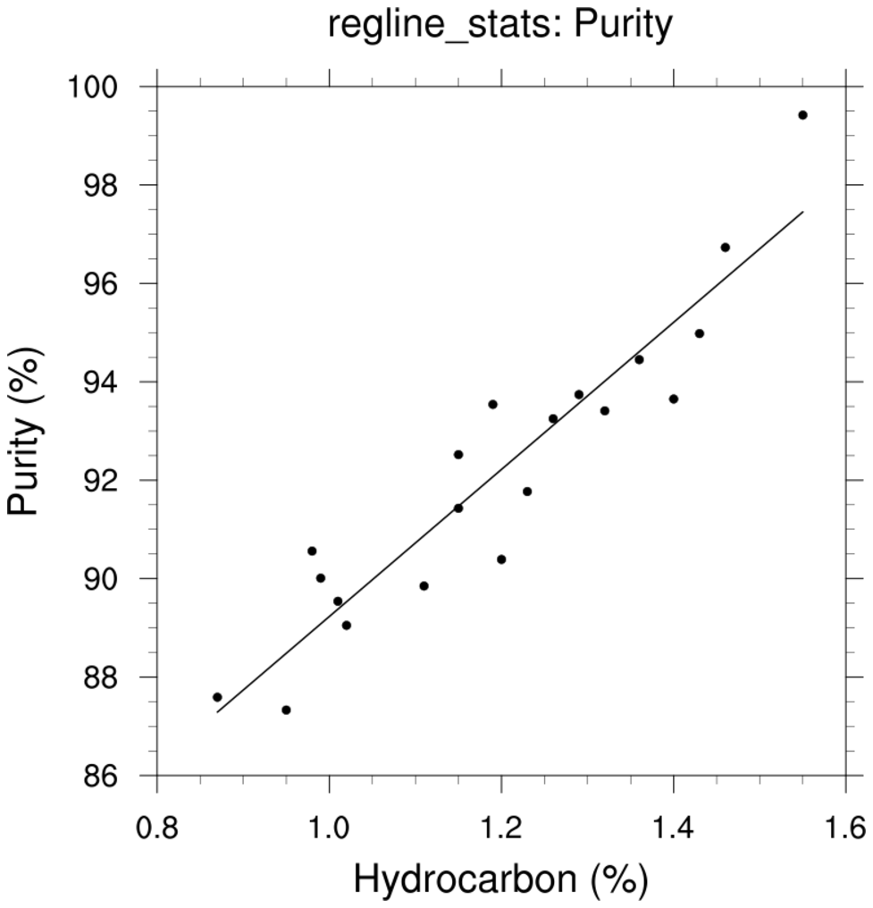
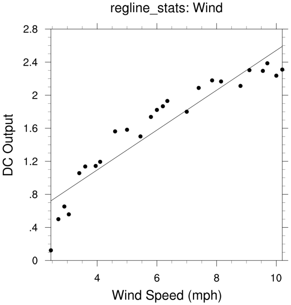
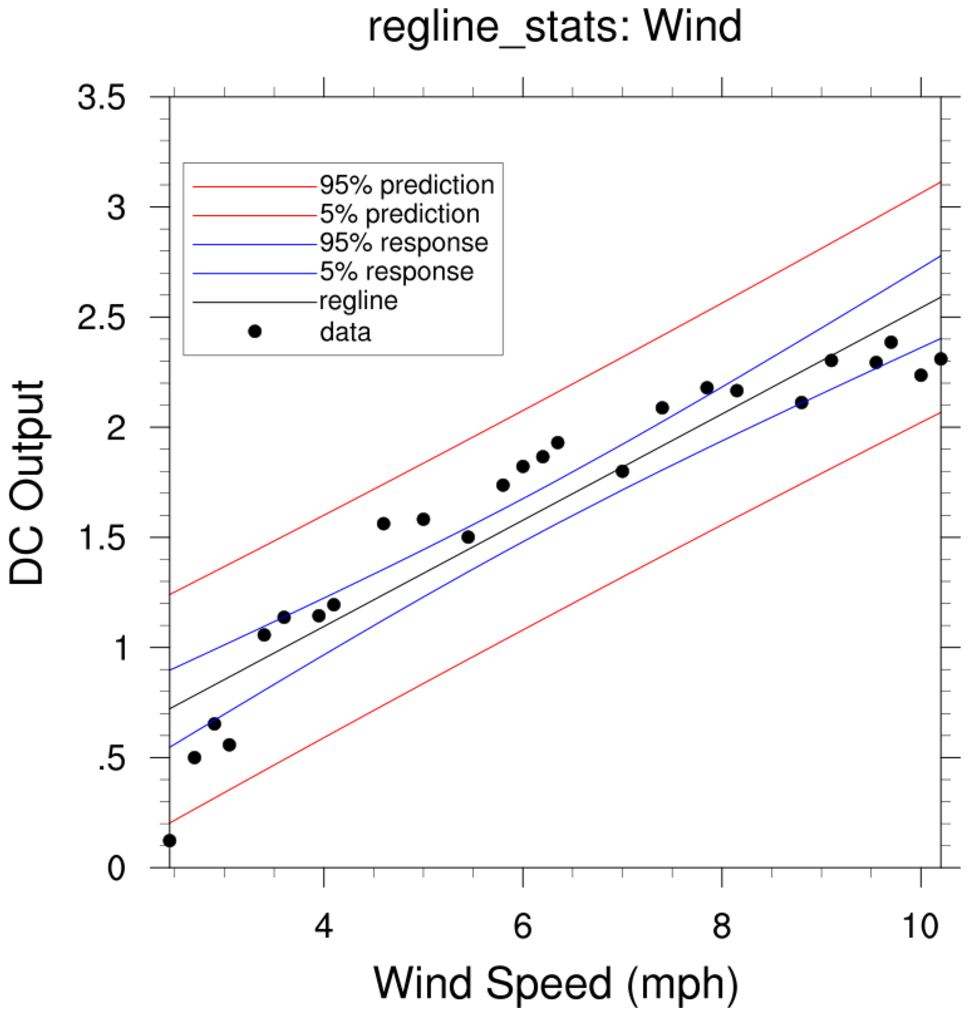
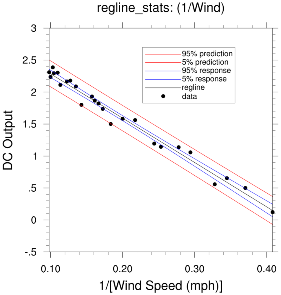
 regress_1c.ncl
:
The reciprocal approach is mentioned at the end of
http://www.stat.ucla.edu/~hqxu/stat105/pdf/ch11.pdf.
R code for processing this is at
http://people.stat.sc.edu/Tebbs/stat509/Rcode_CH11.htm.
The point of this example is that one should examine the residuals from the fitted regression line.
An obvious feature is that the values at the extremes are lower than the fitted line while
the bulk of the middle values are above the fitted line.
It is suggested the the reciprocal (x' = 1/x) be used as the independent variable. The yields
y' = 2.9789 - 6.9345x'
The scatter about the fiited line is reasonably distributed suggesting that the reciprocal transformation
is a better fit than the original model.
 regress_2.ncl
:
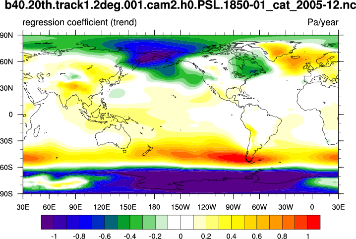
Read sea level pressures (time,lat,lon) over the globe and use
regCoef to calculate the regression coefficients
(aka: slopes, trends). The time units attribute is
"days since 1850-01-01 00:00:00". Hence, the trend units are Pa/day.
These are changed to Pa/year for nicer plot.
 regress_3.ncl
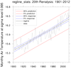
:
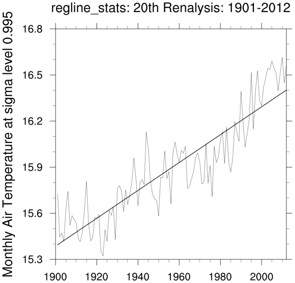
Read northern hemisphere near-surface temperatures spanning 1901-2012
from the 20th Century Reanalysis. Calculate the areal weighted annual mean temperature
for each year. Use
reg_multlin_stats
to calculate the trend and other statistics. Note:
regline
could also have been used for the regression coefficient.
 regress_4.ncl
:
Read northern hemisphere near-surface temperatures spanning 1951-2010
from the 20th Century Reanalysis. Calculate the areal weighted annual mean temperature
for each year. Use
regCoef to calculate the trends.
 regress_5.ncl
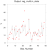
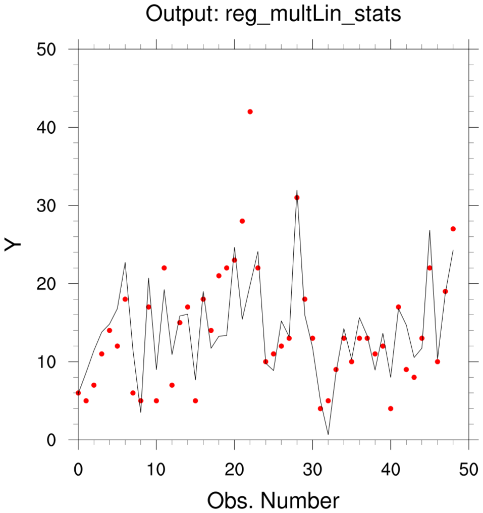
:
Read data from a table and perform a multiple linear regression using
reg_multlin_stats.
There is one dependent variable [y] and 6 predictor variables [x].
Details of the "KENTUCKY.txt" data can be found at:
Davis, J.C. (2002): Statistics and Data Analysis in Geology
Wiley (3rd Edition), pgs: 462-482
The output includes:
[snip]

(0)     ------- ANOVA information--------
(0)
(0)     SST=2934.82  SSR=1800.7  SSE=1134.12
(0)     MST=59.8943  MSR=300.117  MSE=26.3748 RSE=5.13564
(0)     F-statistic=11.3789 dof=(6,43)
(0)               -------

  r2 :  0.613565               ; explains 61% of variance
  r :   0.783304
  r2a : 0.559644
  fuv : 0.386435
[snip]

  stderr :  ( 11.27078, 0.0109590, 0.008168, 0.175949, 0.020587, 0.0021864, 0.072610 )
  tval :    ( -0.19914, 0.4645738, 2.763535,-1.323133, 3.041301,-0.9319575,-1.605605 )
  pval :    (  0.84307, 0.6445273, 0.008318, 0.192626, 0.003961, 0.3564441, 0.115515 )

(0)     -2.24446               ; y-intercept
(1)      0.0050913             ; partial regression coefficients
(2)      0.0225729
(3)     -0.2328043
(4)      0.0626111
(5)     -0.0020377
(6)     -0.1165836
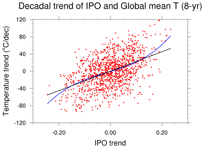
 regress_6.ncl
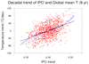
: This is based upon a script created by Aixhu Hu (NCAR).
     (a) Read two text files via asciiread;
     (b) Perform a linear regression using regline;
     (c) Create a 3rd degree polynomial via lspoly_n ;
     (d) Plot markers and the polynomial and regression lines.
Data files:
ipoind_8yrTrend.asc
and
tsind_8yrTrend.asc
The output includes:
    Variable: coef
    Type: float
    Total Size: 16 bytes
                4 values
    Number of Dimensions: 1
    Dimensions and sizes:   [4]
    Coordinates:
    Number Of Attributes: 1
      _FillValue :  9.96921e+36

    (0)     -0.743525
    (1)     180.7366
    (2)     125.8308
    (3)     2630.312
    (0)     ======


    Variable: rc
    Type: float
    Total Size: 4 bytes
                1 values
    Number of Dimensions: 1
    Dimensions and sizes:   [1]
    Coordinates:
    Number Of Attributes: 7
      _FillValue :  9.96921e+36
      yintercept :  -0.08270691
      yave :        -0.14029
      xave :        -0.0002547655
      nptxy :       1175
      rstd :        11.93106
      tval :        18.94417
    (0)     226.024
    (0)     ======
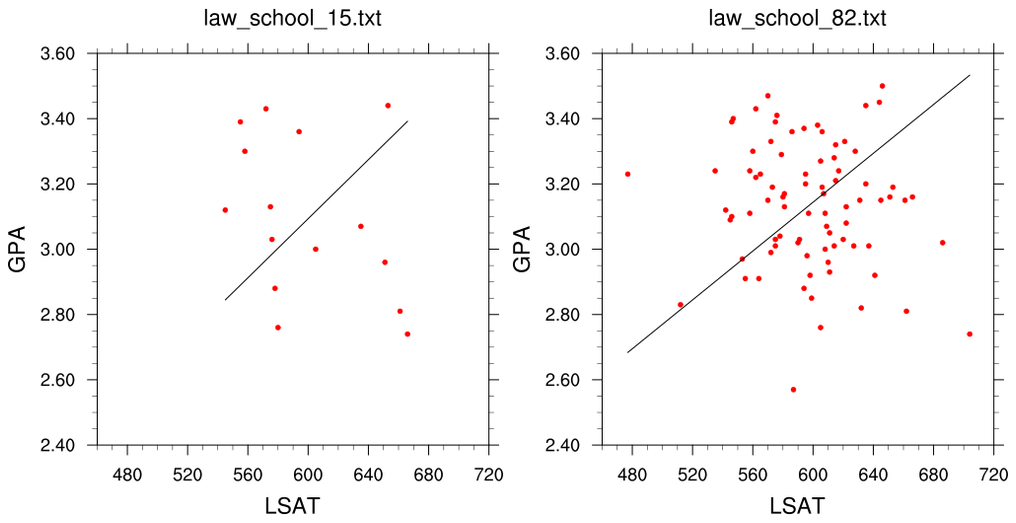
 regress_7.ncl
:
The "Law School Data Sets" (82 school sample and 15-school sample) are used
by several tools (
eg., Matlab and R) for assorted examples.
They are shown here for background purposes because they are used for
some NCL examples also. The data sets are here:
law_school_15.txt
and
law_school_82.txt
Reference: An Introduction to the Bootstrap
           B. Efron and R.J. Tibshirani, Chapman and Hall (1993)
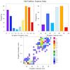
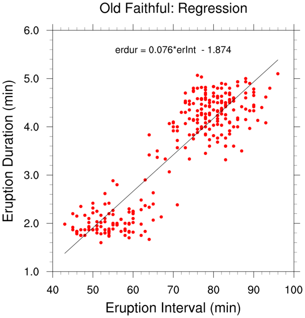
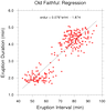 regress_8.ncl
:
The
Old Faithful Geyser Data is used by
R and other tools.
It contains
two variables: (a) the waiting time between eruptions, and
(b) the durations of the eruptions for the
Old Faithful Geyser.
Here, a bivariate linear regression is performed using
regline
and
regline_stats. A comparison to
the output from
R is shown in the examples associated with these functions.
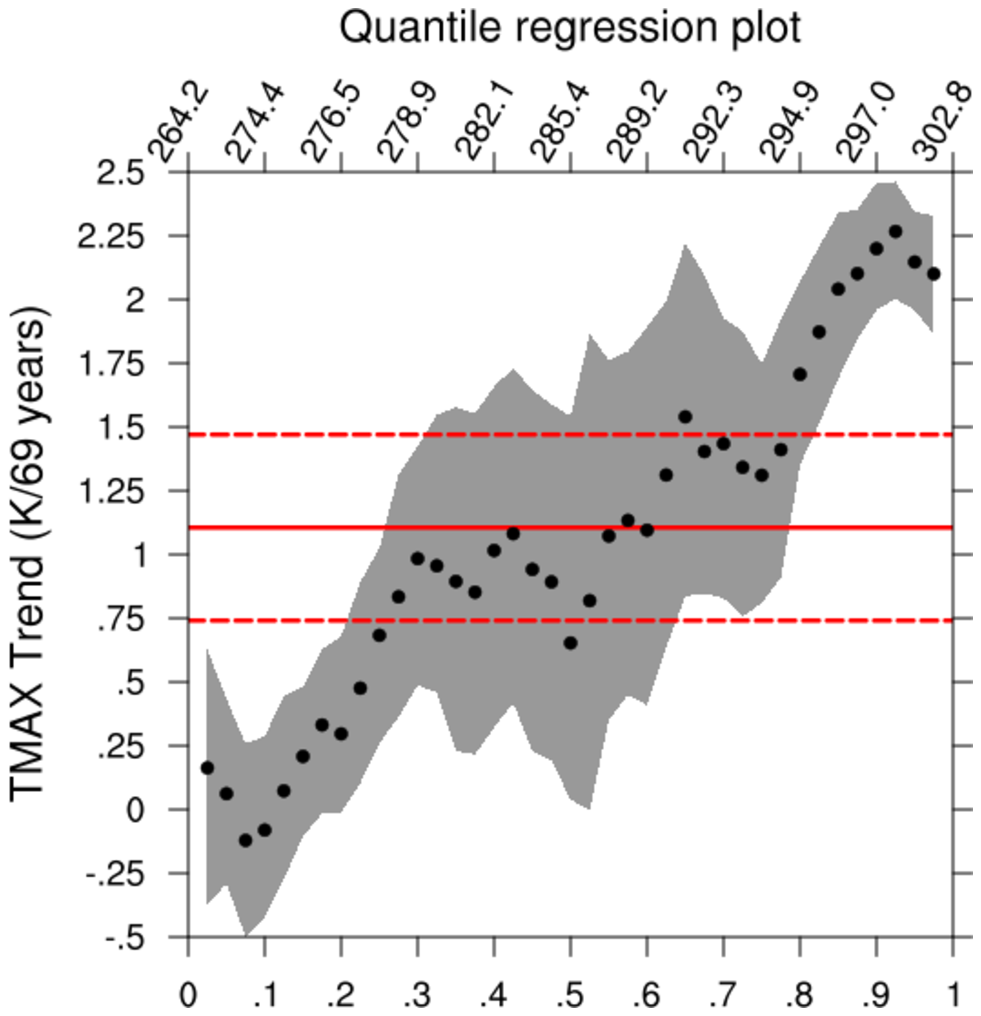
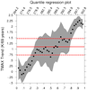 regress_qreg_R.ncl
:
This example, contributed by Laurent Terray [CERFACS; 15 Aug 2018],
illustrates how to invoke an R-function that performs
Quantile
Regression and
Ordinary Least Squares from within an NCL script.
Because it is not possible to
directly pass variables to/from NCL and R,
the script uses files as the method of communication. The files could be any format
that NCL and R can handle (eg: text, binary, netCDF, ...). This example uses
text (csv) files. Specifically, the NCL driver script:
- (a) reads a netCDF file;
- (b) extracts a user specified region of interest using
coordinate subscripting syntax: {...};
- (c) calculates time series of areal means using wgt_areaave_Wrap>;
- (d) creates a csv text file containing the time series of areal means;
- (e) uses system to invoke the R driver script:
QuantReg.R;
- (e1) R function: rq does the quantile regression;
- (e2) R function: ols performs the ordinary least squares fit;
- (f) reads the csv files created by the R driver script;
- (g) use NCL graphics to plot the returned information.
If the R-package "quantreg" is not locally available, it must be installed. Start R:
      > install.packages("quantreg")
      > q()
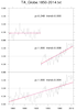 manken_1.ncl
: Read an ascii file
(
TA_Globe.1850-2014.txt; source
(
Met Office Hadley Centre)
and extract pertinent columns. Compute the simple linear regression (
regline_stats; red)
and Mann-Kendall/Theil-Sen (
trend_manken; blue)
trend estimates over three periods. Here, there is virtually no difference between the derived values. Both 'lines' are plotted but only the values from the Mann-Kendall/Theil-Sen are shown. If there are outliers or skewed data, the Theil-Sen is likely to give the better linear trend estimate.
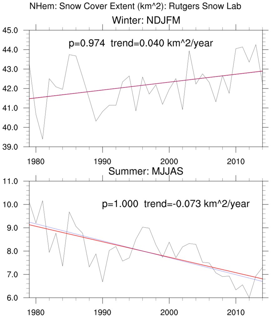
 manken_2.ncl
: Read an ascii file
(
rutgers.snow_cover_extent.time_series.txt; source
(
Rutgers Univ Global Snow Lab)
and extract pertinent columns.
Compute the linear regression and Theil-Sen trend estimates for winter (Nov-Dec-Jan-Feb-Mar) and summer (May-Jun-Jul-Aug-Sep)
over the satellite era (1979-2014).
Both simple linear regression (
regline_stats; red) and Mann-Kendall/Theil-Sen
(
trend_manken; blue) estimates are shown. The summer trend lines illustrate a small difference
between the trend estimates. It is likely that the distribution of residuals about the linear regression line is slightly skewed.
Hence, the Theil-Sen is likely better.


