NCL Home > Documentation > Functions > General applied math

reg_multlin_stats

Performs multiple linear regression analysis including confidence estimates and creates an ANOVA table.

Available in version 6.2.0 and later.

Prototype

load "$NCARG_ROOT/lib/ncarg/nclscripts/csm/contributed.ncl"  ; This library is automatically loaded
                                                             ; from NCL V6.2.0 onward.
                                                             ; No need for user to explicitly load.

	function reg_multlin_stats (
		y [*] : numeric,                                  
		x     : numeric,             [*] or [*][*] only,  
		opt   : logical                                   
	)

	return_val [*] :  float or double

Arguments

A one-dimensional array of length N containing the dependent variable [y(N)].

A one dimensional array of size N or a two-dimensional array of size [(N,M)] where M is the number of independent variables. See the Description section below for more comments.

opt

A logical variable. If opt=True, then the following attributes can be set:

   
   opt = True
   opt@print_data  = True     ; will print the input data in table form
   opt@print_anova = True     ; will print the ANOVA table

Return value

The one-dimensional array, say b, returned is size (M+1). This will contain the y-intercept and the partial regression coefficients associated with each independent variable. In addition, many statistical quantities are returned as attributes of b.

The return values will be of type double if x or y is double, and float otherwise.

Description

reg_multlin_stats performs a multiple linear regression. A one dimensional array (call it b(M+1)), containing the y-intercept and the partial regression coefficients is returned. The coefficients represent the rate of change in the dependent variable for a unit change in the independent variable, under the constraint that all other independent variables are held constant.

The input argument x for the function reg_multlin_stats differs from that input to the builtin function reg_multlin. The builtin function requires the user to create a 'design matrix' which consists of a 'dummy' column of 1s and the independent variables. This is a bit cumbersome. This function requires only the independent variables be input. The function creates the required 'design matrix' internally.

The partial regression coefficients, b, can be used to calculate standardized regression coefficients, say B. The B represent the partial regression coefficients in units of standard deviation. The following illustrates the simple calculation needed make the transformation:

    B(j) = b(j)*standard_deviation(X(j))/standard_deviation(Y)

Since the B are expressed in units of standard deviation they may be directly compared with each other to determine the most effective variables.

The user may wish to take into account the uncertainty associated with each estimated parameter and the overall uncertainty. This information is returned as the attributes stderr, tval and pval. In addition, an ANalysis Of VAriance [ANOVA] table is returned in the form of attributes (see example).

While missing values are allowed, it is recommended that users not input any missing independent values. It just confuses the results. Missing values should be indicated by the _FillValue attribute.

Examples

Example 1

The following is from http://reliawiki.org/index.php/Multiple_Linear_Regression_Analysis


   load "$NCARG_ROOT/lib/ncarg/nclscripts/csm/contributed.ncl"

   y    = (/251.3, 251.3, 248.3, 267.5, 273.0, 276.5, 270.3, 274.9, 285.0 \
          , 290.0, 297.0, 302.5, 304.5, 309.3, 321.7, 330.7, 349.0 /)

   x1   = (/ 41.9,  43.4,  43.9,  44.5,  47.3,  47.5,  47.9,  50.2,  52.8 \
           , 53.2,  56.7,  57.0,  63.5,  65.3,  71.1,  77.0,  77.8 /) 

   x2   = (/ 29.1,  29.3,  29.5,  29.7,  29.9,  30.3,  30.5,  30.7,  30.8 \
           , 30.9,  31.5,  31.7,  31.9,  32.0,  32.1,  32.5,  32.9 /)
   nrow = dimsizes(y)

   np   = 2
   xp   = new( (/nrow,np/), typeof(x1))  ; create an array to hold predictor variables   
   xp(:,0) = x1
   xp(:,1) = x2
           
   opt = True
   opt@print_anova = True     ; optional
   opt@print_data  = True
   b   =  reg_multlin_stats(y,xp,opt) ; partial regression coef
   print(b)

Partial regression coefficients (b) and additional statistics are returned.

Setting print_data=True resulted in the input data being printed as a table.

----- reg_multlin_stats: Y, XP -----
  
     251.30      41.90      29.10
     251.30      43.40      29.30
     248.30      43.90      29.50
     267.50      44.50      29.70
     273.00      47.30      29.90
     276.50      47.50      30.30
     270.30      47.90      30.50
     274.90      50.20      30.70
     285.00      52.80      30.80
     290.00      53.20      30.90
     297.00      56.70      31.50
     302.50      57.00      31.70
     304.50      63.50      31.90
     309.30      65.30      32.00
     321.70      71.10      32.10
     330.70      77.00      32.50
     349.00      77.80      32.90

Setting print_anova=True resulted in the ANOVA information being printed:


        ------- ANOVA information-------- 
        SST=13239.7  SSR=12816.4  SSE=423.372
        MST=827.483  MSR=6408.18  MSE=30.2409 RSE=5.49917
        F-statistic=211.904 dof=(2,13)
                 -------

The print(b) yielded the following (edited) output. All the comments were manually added.


       Variable: b
       Type: float
       Total Size: 12 bytes
                   3 values
       Number of Dimensions: 1
       Dimensions and sizes:   [3]
       Coordinates: 
       Number Of Attributes: 27
         _FillValue :  9.96921e+36
         long_name :   multiple regression coefficients
         model :       Yest = b(0) + b(1)*X1 + b(2)*X2 + ...+b(M)*XM
       
         N :   17                              ; # of observations
         NP:   2                               ; # of predictor variables
         M :   3                               ; # of returned coefficients
         bstd : (  0, 0.5029772, 0.4922954 )   ; standardized partial regression coefficients 
                                               ; [ignore 1st element]

                                               ; ANOVA information: SS=>Sum of Squares
         SST : 13239.72                        ; Total SS:      sum((Y-Yavg)^2) 
         SSE : 423.3723                        ; Residual SS:   sum((Yest-Y)^2)
         SSR : 12816.36                        ; sum((Yest-Yavg)^2)
         MST : 827.4825
         MSE : 30.24088
         MSE_dof :     14
         MSR : 6408.178

         RSE : 5.499171                        ; residual standard error; sqrt(MSE)
         RSE_dof :     13

         F     :   211.9045                    ; MSR/MSE
         F_dof :   ( 2, 14 )
         F_pval:  3.419033e-11

         r2  :  0.9680232                      ; square of the Pearson correlation coefficient 
         r   :  0.9838817                      ; multiple (overall) correlation: sqrt(r2)
         r2a :  0.9634551                      ; adjusted r2... better for small N

         fuv : 0.03197682                      ; (1-r2): fraction of variance of the regressand 
                                               ; (dependent variable) Y which cannot be explained,
                                               ;  i.e., which is not correctly predicted, by the 
                                               ; explanatory variables X.

         Yest : [ARRAY of 17 elements]         ; Yest = b(0) + b(1)*X1 + b(2)*X2 

         stderr :      ( 100.8641, 0.3945341, 3.931675 )       ; std. error of each b
         tval :        ( -1.521964, 3.139713, 3.073079 )       ; t-value 
         pval :        ( 0.1502808, 0.007238129, 0.008262509 ) ; p-value
       
       (0)  -153.5115                          ; partial regression coef: b
       (1)     1.238724
       (2)    12.08235

These results match R exactly:


       df = read.table("./ReliaWiki.txt", header=TRUE)
       dim(df)
     [1] 17  3
     
       names(df)
     [1] "Y"  "X1" "X2"
     
       mlr <- lm(Y~., data=df)
       summary(mlr)
     
     Call:
     lm(formula = Y ~ ., data = df)
     
     Coefficients:
                  Estimate Std. Error t value Pr(>|t|)   
     (Intercept) -153.5117   100.8799  -1.522  0.15034   
     X1             1.2387     0.3946   3.139  0.00724 **
     X2            12.0824     3.9323   3.073  0.00827 **
     ---
     Signif. codes:  0 ***, 0.001 **, 0.01 *, 0.05  . 
     
     Residual standard error: 5.499 on 14 degrees of freedom
     Multiple R-squared:  0.968,     Adjusted R-squared:  0.9635 
     F-statistic: 211.9 on 2 and 14 DF,  p-value: 3.419e-11

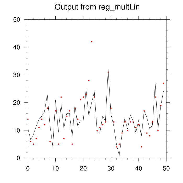
Example 2: Read tabular data from a file. The data is from:
Davis, J.C. (2002): Statistics and Data Analysis in Geology, Wiley (3rd Edition) See pg: 462-482

A scatter plot of the data and the resultant fit is here.


       load "$NCARG_ROOT/lib/ncarg/nclscripts/csm/contributed.ncl"

       diri    = "./"
       fili    = "KENTUCKY.TXT"
       
       ncol    = numAsciiCol(diri+fili)
       data    = readAsciiTable( diri+fili, ncol, "float" , 1)  ; one header 

       y       = data(:,0)
       x       = data(:,1:)

       opt = True
       opt@print_anova = True

       b    =  reg_multlin_stats(y,x,opt) ; partial regression coef
       print(b)