NCL Home > Documentation > Functions > General applied math

bw_bandpass_filter

Applies a Butterworth bandpass filter optimized for narrow bandwidths to time series.

Available in version 6.3.0 and later.

Prototype

	function bw_bandpass_filter (
		x        : numeric,  
		fca  [1] : numeric,  
		fcb  [1] : numeric,  
		opt  [1] : logical,  
		dims [*] : integer   
	)

	return_val  :  float or double, see return value description below

Arguments

An array of time series to be filtered. Missing values are not allowed.

fca

A scalar indicating the cut-off frequency of the ideal band pass filter: (0.0 < fca < 0.5).

fcb

A scalar indicating the cut-off frequency of the ideal band pass filter: (0.0 < fcb < 0.5) and (fcb > fca).

opt

If opt = True, five attributes are available:

opt@m - order of filter; 4 <= m <= 6 should be adequate for most applications. Currently, the maximum value allowed is 10. Default is 6.
opt@dt - a scalar specifying the sampling interval. Default is 1.0.
opt@remove_mean - a logical scalar whether to remove the mean. Default is True.
opt@return_filtered - a logical scalar whether to return the filtered time series values. Default is True.
opt@return_envelope - a logical scalar whether to return the envelope time series values. Default is False.

dims

The dimension(s) of x on which to apply the filter. Must be consecutive and monotonically increasing.

Return value

If both opt@return_filtered and opt@return_envelope are True, the returned array will be of size (2,dimsizes(x)).

Otherwise, if only one of opt@return_filtered or opt@return_envelope are True, the returned array will be of the same size and shape as x.

The return type will be double if x is double, and float otherwise.

Description

The following is an edited description extracted from the underlying code.

The bw_bandpass_filter executes a fast, stable zero phase Butterworth bandpass filter of order (m), which is optimized for narrow band. Stability of the method is achieved by reducing the bandpass filter calculations to simple cascaded first order filters, which are forward and reverse filtered for zero phase. The method also does a linear shift of a Butterworth lowpass filter to an equivalent bandpass, without going through a standard non-linear translation to bandpass. An option is included to remove the signal mean initially to compensate for large DC offsets.

An advantage of the Butterworth bandpass filter is that there is no loss of data at the beginning and end.

Reference:

    Electronic Supplement to Development of a Time-Domain, Variable-Period 
    Surface Wave Magnitude Procedure for Application at Regional and 
    Teleseismic Distances, Part I: Theory; David R. Russell
    Bulletin of the Seismological Society of America

    http://www.seismosoc.org/publications/BSSA_html/bssa_96-2/05055-esupp/

                  i              band pass
             1.0  i           |------------|      
                  i           |            | 
                  i           |            |   
                  i           |            |     
                  i           |            |           
             0.0  i___________|____________|_______________
                 0.0          |            |           0.5
                             fca          fcb

Examples

See Butterworth filter examples.

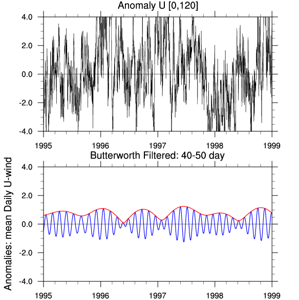
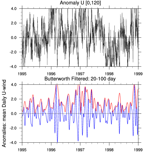
Example 1: Perform optimized Butterworth band pass (40-50 day) filter on daily data at a specific location.


    LAT    = 0          ; arbitrary
    LON    = 120

    diri  = "./"
    fili  = "uwnd.day.850.anomalies.1980-2005.nc"
    fi    = addfile(diri+fili, "r")
    ua    = f->U_anom(:,{LAT},{LON})            ; ua(time)    ; read from one grid point

    ca    = 50.0        ; band start (longer period)
    cb    = 40.0        ; band end

    fca   = 1.0/ca      ; 'left'  frequency
    fcb   = 1.0/cb      ; 'right' frequency

    dims  = 0           ; 'time' dimension  

    opt   = True        ; options to set
    opt@return_envelope = True ; time series of filtered and envelope values

    ua_bf = bw_bandpass_filter (ua,fca,fcb,opt,dims)       ; (ua,fca,fcb,opt,dims)
    copy_VarMeta(ua, ua_bf)
    ua_bf@long_name = "Band Pass: "+cb+"-"+ca+" day"

    printVarSummary(ua_bf)

The (edited) ua_bf output looks like:


Variable: ua_bf 
Type: float
Number of Dimensions: 2
Dimensions and sizes:   [2] x [time | 9497] 
Coordinates: 
            time: [17347584..17575488]
Number Of Attributes: 5
  units :       m/s
  long_name :   Band Pass: 40-50 day
  _FillValue_original : 32766
  lat :  0
  lon : 120

Time series plots depicting the bandpass and associated envelope series for two different pass bands follow: TOP: the original time series; BOTTOM: the bandpass (blue) and the envelope series (red).

40-50 day
20-100 day

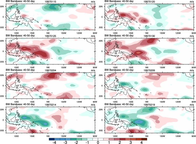
Example 2: Perform optimized Butterworth band pass filter to a narrow band of daily data at multiple locations (grid points).

   latS   = -20.0
   latN   =  20.0

    diri  = "./"
    fili  = "uwnd.day.850.anomalies.1980-2005.nc"
    fi    = addfile(diri+fili, "r")
    ua    = f->U_anom(:,{latS:latN},:)   ; (time,lat,lon) dim number => (0,1,2)

    ca    = 50.0        ; band start (longer period)
    cb    = 40.0        ; band end

    fca   = 1.0/ca      ; 'left'  frequency
    fcb   = 1.0/cb      ; 'right' frequency

    opt   = False       ; use default options (time series of filtered
                        ; values will be returned)

    ua_bf = bw_bandpass_filter (ua,fca,fcb,opt,0)   ; (ua,fca,fcb,)
    copy_VarMeta(ua, ua_bf)
    ua_bf@long_name = "BW Bandpass: "+cb+"-"+ca+" day"

    printVarSummary(ua_bf)