NCL: Filters

Reference:

    Electronic Supplement to Development of a Time-Domain, Variable-Period 
    Surface Wave Magnitude Procedure for Application at Regional and 
    Teleseismic Distances, Part I: Theory; David R. Russell
    Bulletin of the Seismological Society of America

    http://www.seismosoc.org/publications/BSSA_html/bssa_96-2/05055-esupp/

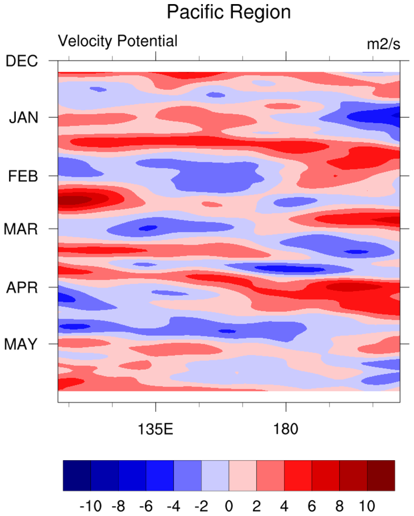
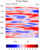filter_1.ncl: Reads in a variable from a netCDF file, averages all latitudes between 15S and 15N, applies a user specified filter on the "time" dimension, and creates a color Hovmueller diagram.

gsn_csm_hov is the graphical interface that creates Hovmueller diagrams.

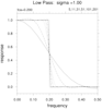
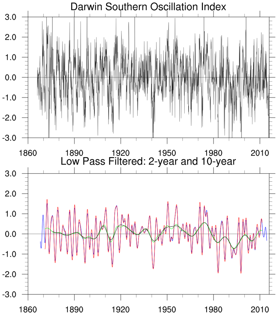
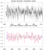filters_2.ncl: Low pass filters via filwgts_lanczos:

• Read the monthly Southern Oscillation Index (Darwin only)
• Using different filter lengths (49 [solid], 121 [dashed]), generate two low pass filters that (ideally) will remove fluctuations less than 24 months (2 years).
• Using different filter lengths (121 [solid], 241 [dashed]), generate two low pass filters that (ideally) will remove fluctuations less than 120 months (10 years).

The blue (49 weights) and red (121 weights) curves are for the 24-month filter. In this case, not much was gained by using much longer filter (121 vs 49). Also, using the 49-point filter returned more data at the ends.

The green (121 weights) and black (241 weights) curves are for the 120-month filter. The response functions are not much different and, as a result, the decadal curves are not much different.

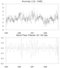
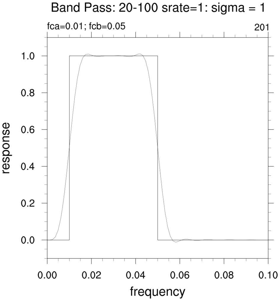
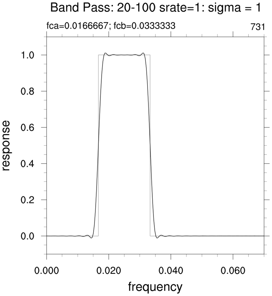
filters_3.ncl: Band pass filters via filwgts_lanczos:

Generate and apply a 20-100 day band pass filter using 201 weights. The response function for the filter is also shown.

The Lanczos filter weights are applied to the entire daily series spanning 1980-2005. The plotted values do not have any missing points 'end-points' because the plotted time period (1995-1998) is a subset of the entire series.

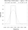
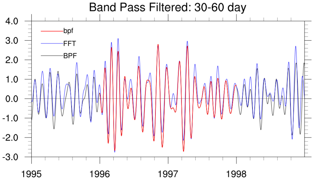
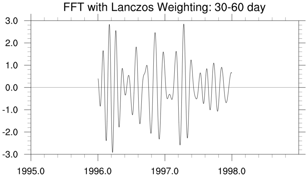
filters_4.ncl: Comparison: band pass filters via filwgts_lanczos and via FFT:

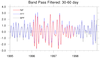
This example compares results returned using filwgts_lanczos and FFTs [ezfftf and ezfftb]. The band pass period for this example is 30-to-60 days. The FFT filtering is performed by applying a 'boxcar' cutoff in frequency space (1/30 and 1/60) while the Lanczos weights are applied in time. The Lanczos band pass filter in this example is 731 points. This means that exactly one year of data will be 'lost' at the beginning and end of the series to which the Lanczos filter is applied.

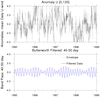
(a) Read entire 1980-2005 daily anomaly data [here, anomolous zonal wind] 
    for a specific location [0,100E]
(b) Apply the Lanczos filter weights to the entire 1980-2005 series. The loss
    of data at the end points will affect 1980 and 2005. [BPF, black line]
(c) Select a four year [1995-1998] temporal window to demonstrate
    how using a segment of an infinitely long [well, ok, 1980-2005 :-) ]
    would compare.
(d) Apply the Lanczos filter to the 4-year temporal window only. The filtered
    series for 1995 and 1998 will be set to missing. [bpf, red line]
(e) Perform a Fourier analysis (ezfftf) on the input anomalies for the 
    4-year temporal window; set the Fourier coefficents outside the 
    desired frequency band to zero (boxcar); perform a Fourier synthesis (ezfftb) 
    to return to temporal window space. [FFT, blue line]
    For simplicity, no tapering (taper) or detrending (dtrend) was performed. 

If the BPF line is considered "truth", then, in this case (a fairly broad band pass), the FFT approach yields similar results to the BPF over the temporal window subperiod. There are some minor phase differences outside at the 'ends' and one issue in 1997 but, overall, pretty good agreement. In addition, there is apparently no loss of data at the beginning and end of the sub-period. Why not use the FFT approach all the time? If the number of weights had been kept the same, but the band pass period was much shorter, then the fourier synthesis would likely show more distinct differences.

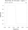
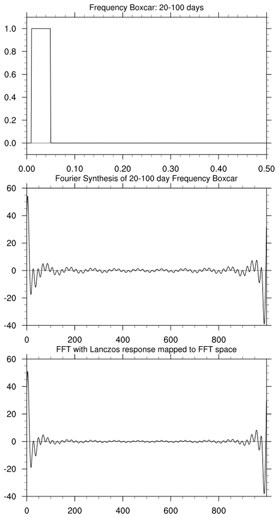
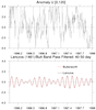
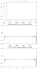
filters_5.ncl: Band pass filters via FFTs: End point problems:

This demonstrates one 'problem' with using boxcar type truncation of Fourier coefficients in the frequency domain. Consider a series of length N (here, N=1000 days) which will have N/2 frequencies (0 to 0.5 cycles/day). In this example, the 20-100 day band pass period suggested by MJO Clivar will be used.

(a) Create Fourier coefficients (real and imaginary) which are 1.0 in the 
    frequency band of interest and 0.0 elsewhere. This is the boxcar response in 
    frequency space (top figure).  In temporal space, it would take an infinite 
    number of weights to yield the boxcar frequency response. 
(b) Perform a Fourier synthesis (ezfftb) on (a) to return to temporal 
    space (middle figure).
(c) Generate Lanczos weighting using 201 weights; 'map' the Lanczos response function into FFT 
    frequency space via linear interpolation; apply the mapped weights to the
    boxcar Fourier coefficients in the frequency domain; perform a Fourier 
    synthesis (bottom figure).

The middle figure shows that a Fourier synthesis of the boxcar Fourier coefficients yields spurious and significant 'end-effects' and, in this idealized case, minor ripples at all times. In the real world, the real and imaginary coefficients are not all equal [here, 1.0], the synthesis can have additional unwanted effects. The reconstructed series can reflect local and, possibly, significant (in time) occurring features.

Is there a way to use an FFT and get the desirable and predictable characteristics Lanczos weighting? Weighting the boxcar Fourier coefficients by the Lanczos responses yields slightly smaller ripples and end-effects (bottom figure).

Punch line: The Fourier approach yields values but you are not quite sure of what you are getting. At least with the Lanczos filter approach, you know what you are getting.

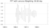
filters_6.ncl: FFT speed and Lanczos clarity:

(a) Develop a Lanczos filter that has good characteristics
(b) Map the Lanczos response function into FFT frequency space 
    via linear interpolation
(c) Apply the mapped weights to the Fourier coefficients.
(d) Perform the Fourier synthesis.
(e) In the time domain, manually set the end-points to missing. 
    There is no way around this!!!!

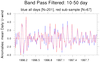
filters_7.ncl: Matching data with different sampling intervals.

A user had daily data which was treated with a 10-50 day band pass filter. A different series was availble but values were available every 3rd day. How to create a filter that will operate on the latter series which will 'match' that used on the daily data. (See the above comments by Dave Allured.)

The figure shows a comparison. Do they match exactly? Of course not! (a) Information was lost by sampling every 3rd day. There is no way to recover this lost information; (b) the sereies are not plotted at the exact same time points.

Does the new filtered series capture the essentials of the fully samples series? Yes!

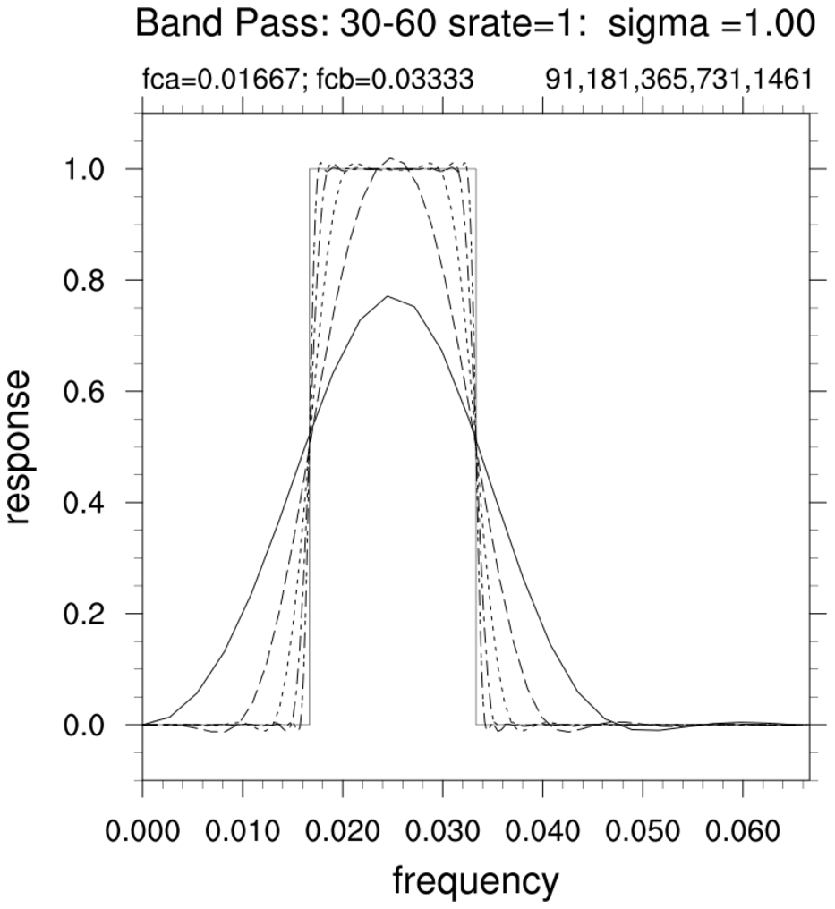
filters_8.ncl: Lanczos Response Functions

This script will generate one or more response functions for different Lanczos filter lengths. This allows users to assess which filter length is acceptable for their application. There is a trade-off amongst bandwidth, filter length and response.

This example was run twice to get the 2 figures.

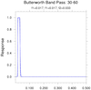
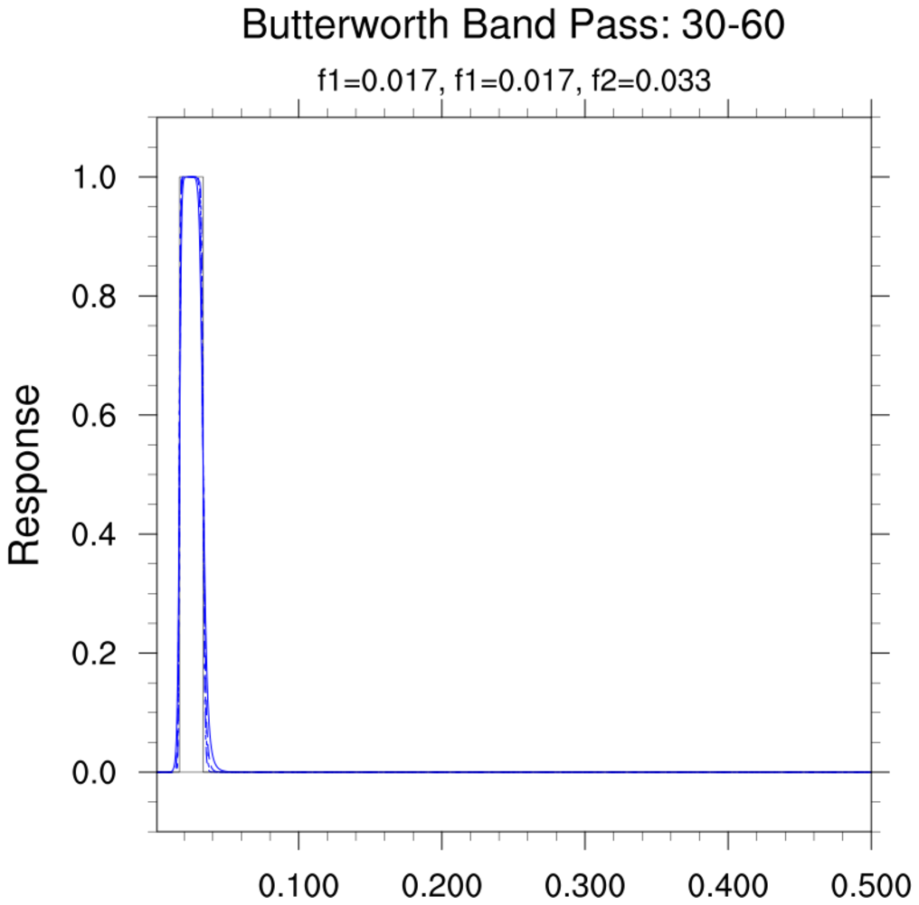
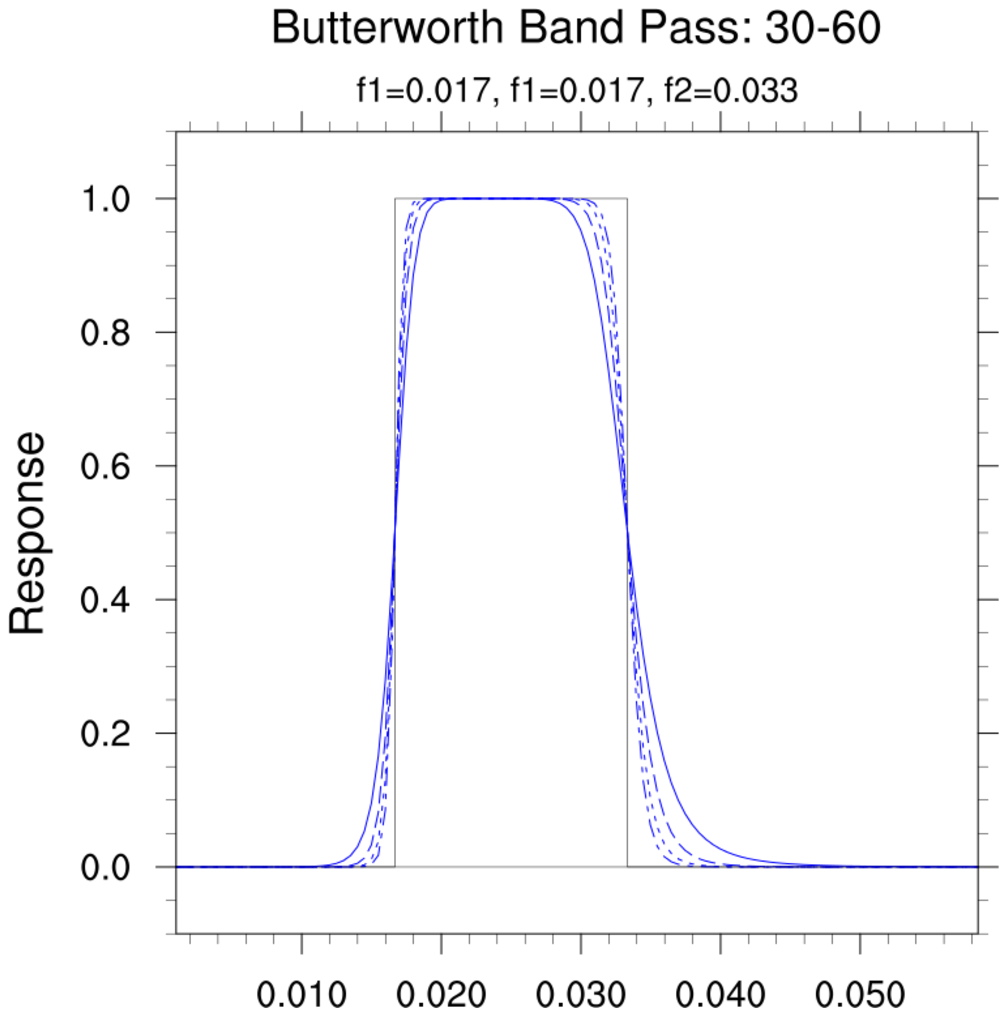
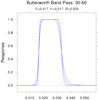filters_9.ncl: Butterworth Response Functions (V6.3.0)

This script will generate one or more response functions for different Butterworth pole values. The left figure shows the bandpass relative to the full frequency span. The right figure shows a blowup of the region of interest.

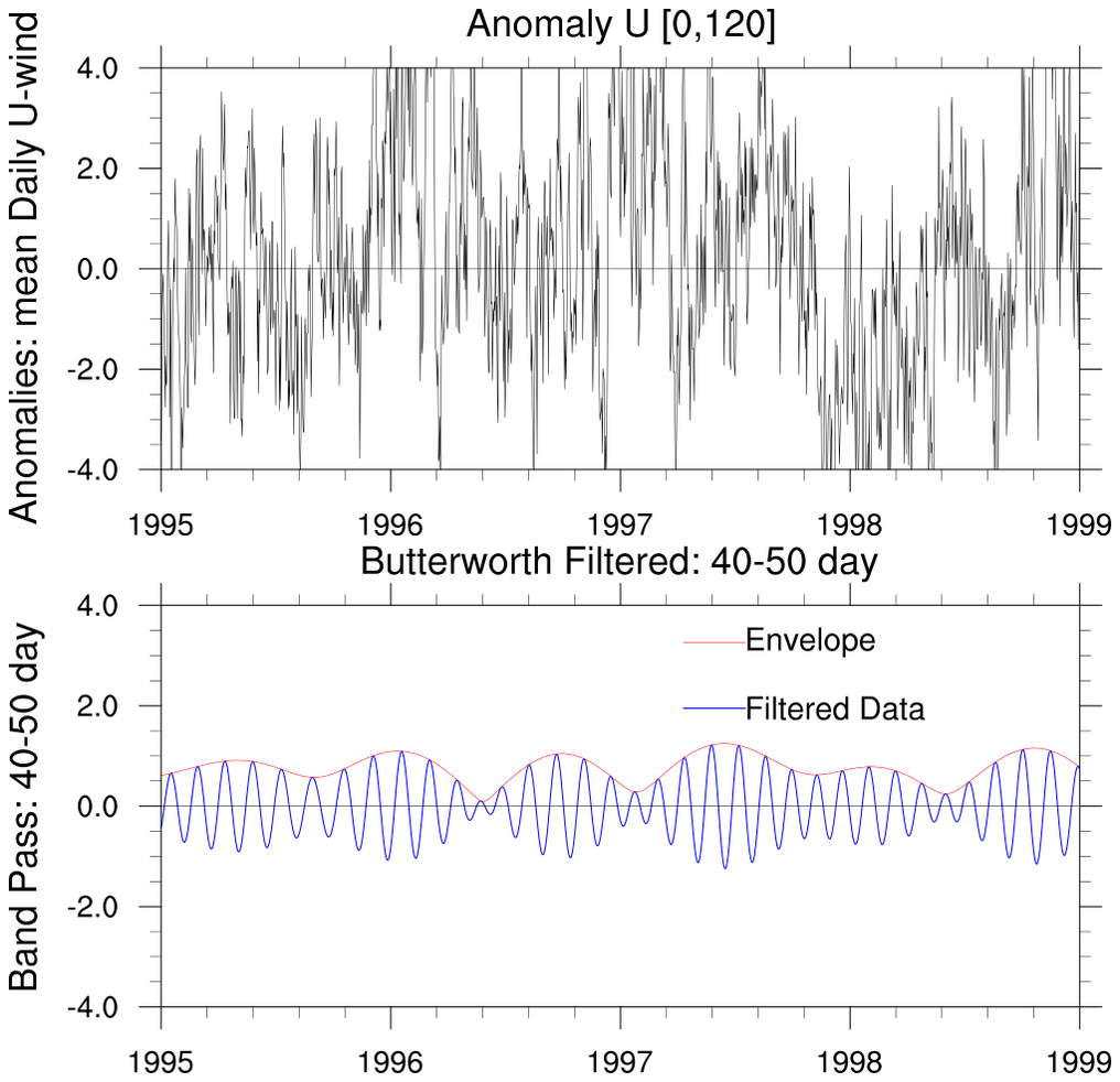
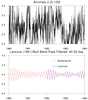
bfband_1.ncl: This script reads a time series at a user specified grid point. It applies a Butterworth band Pass filter (bw_bandpass_filter) to the series. The raw (top) and filtered/envelope (bottom) series illustrates usage and results.

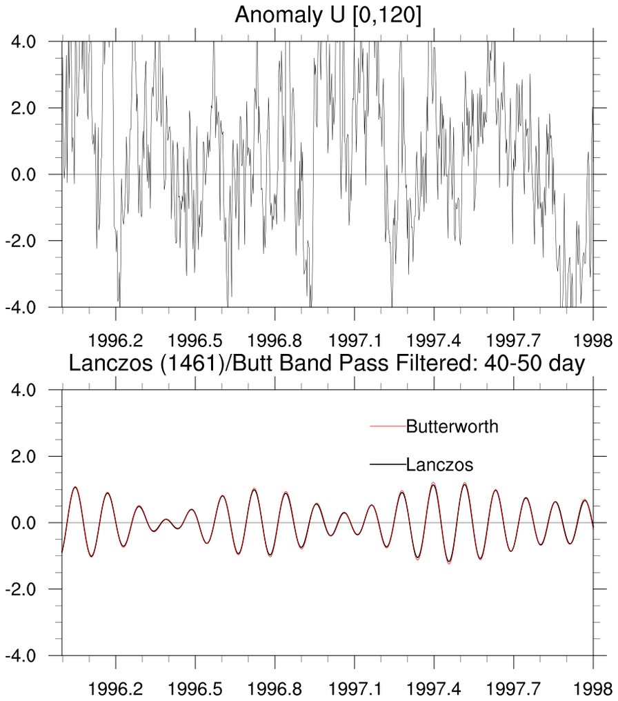
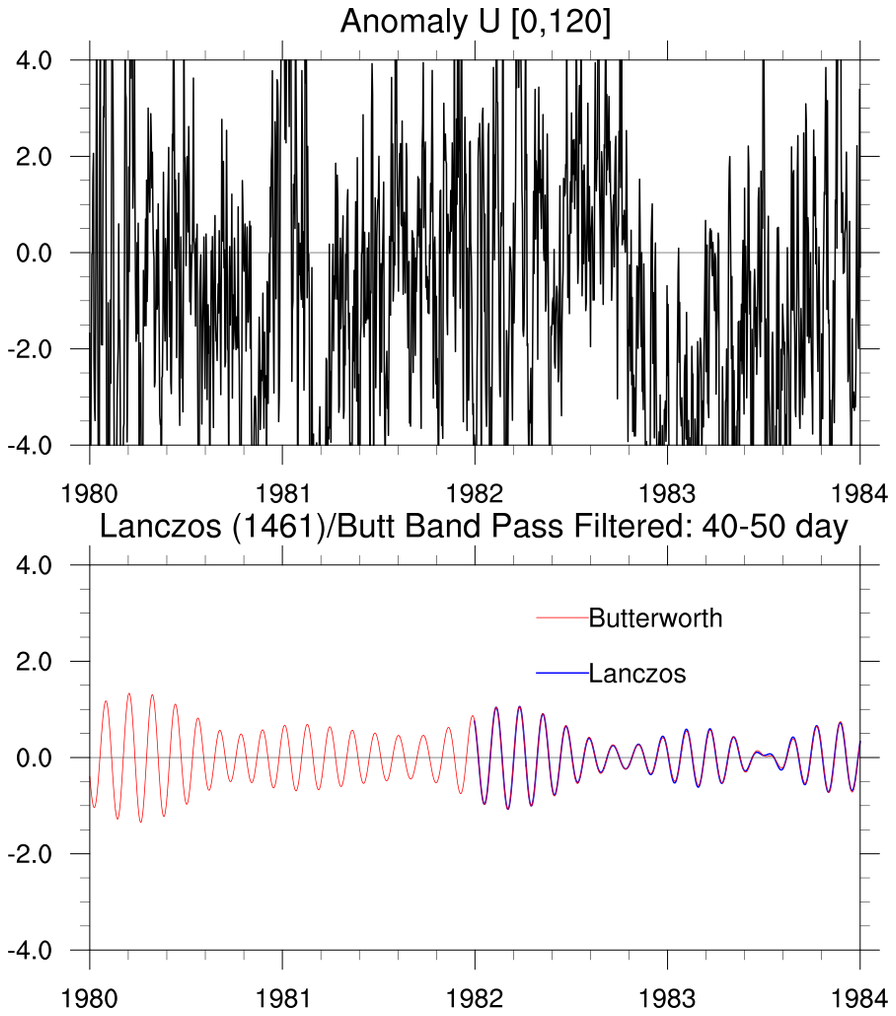
bfband_2.ncl: Use Lanczos filter (filwgts_lanczos) with 1461 weights (=4*365+1) to filter a long time series. Basically 2 years of daily data are lost at each end of the series. Also, apply a Butterworth filter (bw_bandpass_filter). No data are lost. The rightmost figure shows the beginning of the full time series.

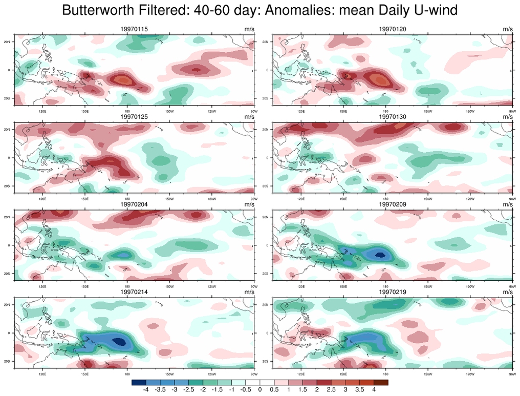
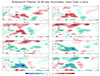
bfband_3.ncl: Plot spatial patterns of 40-50 day Butterworth band passed data every 5 days.