NCL Graphics: Pressure/Height vs. Latitude (high-level plot interface)

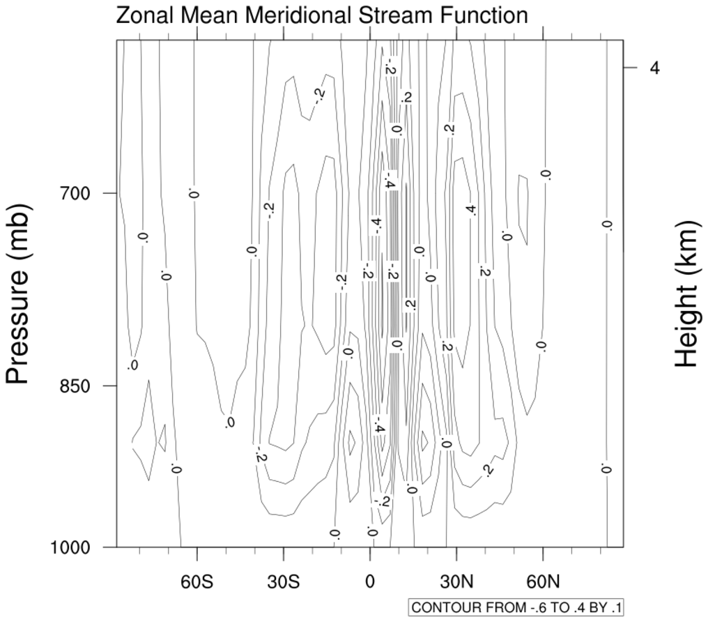h_lat_1.ncl: Calculates the mean meridional stream function via the function zonal_mpsi and creates a simple height versus latitude plot.

gsn_csm_pres_hgt is the plot interface that plots height versus latitude plots.

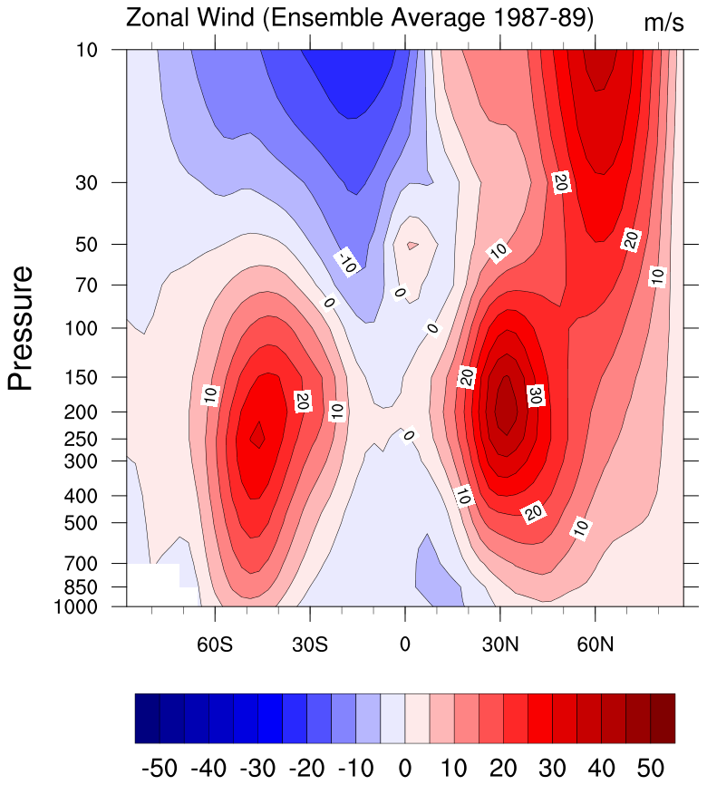
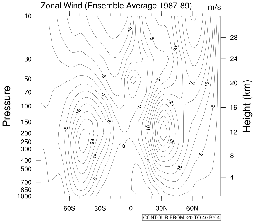h_lat_2.ncl: Another simple default plot of U versus height and latitude.

Note, this data is already on pressure levels. If this were model data, it would be necessary to interpolate from the hybrid coefficients to pressure levels.

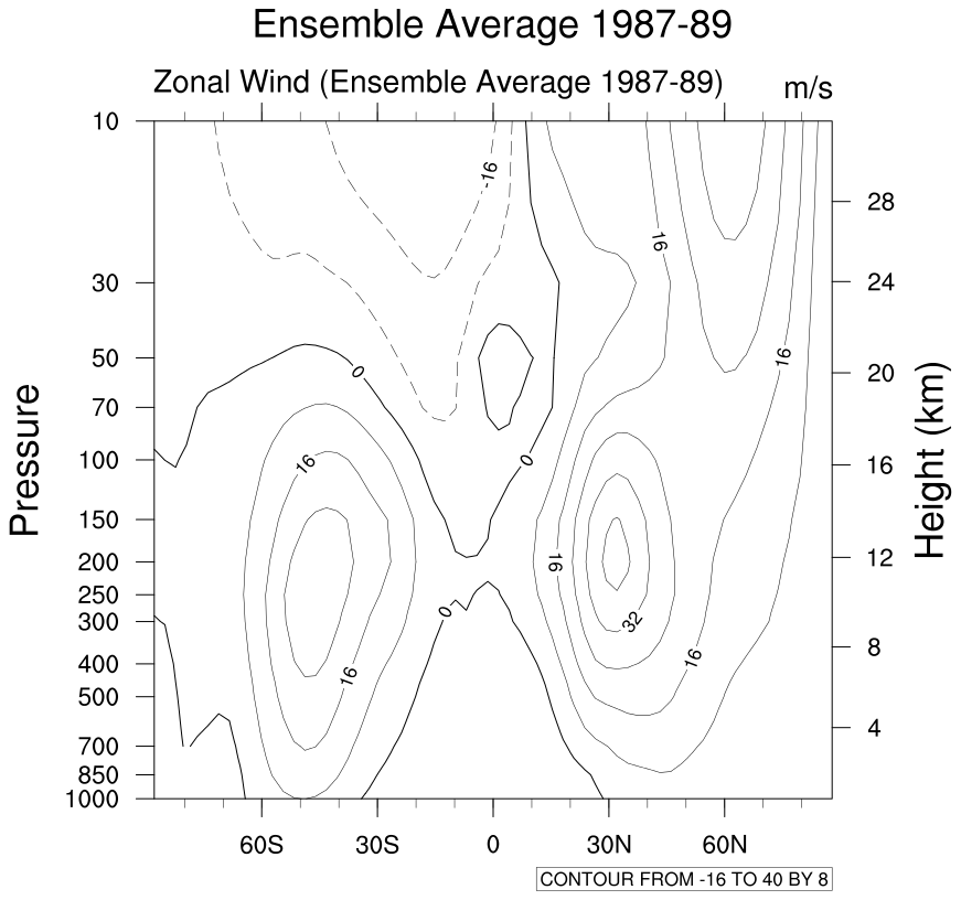
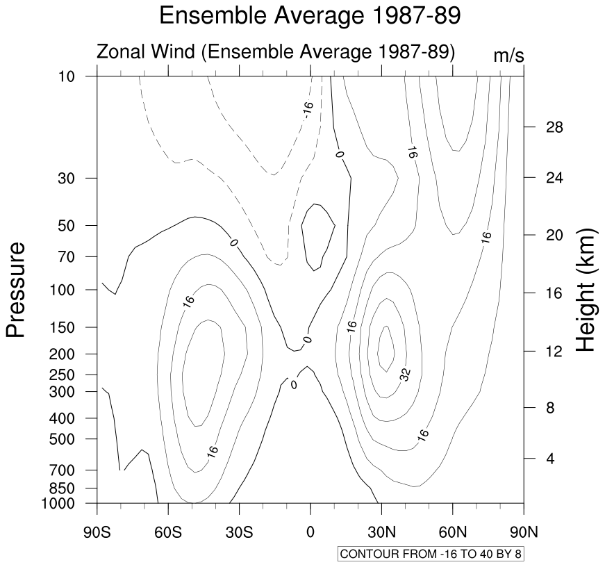h_lat_3.ncl: The first plot creates a double thick line at the zero contour and dashed negative lines. The second plot demonstrates adding latitudinal labels to 90 degrees.

gsnContourZeroLineThicknessF doubles the thickness of the zero contour, gsnContourPosLineDashPattern dashes the positive contours (not used here), and gsnContourNegLineDashPattern dashes the negative contours.

add90LatX is the shea utility function that creates latitude labels to a full 90 degrees.

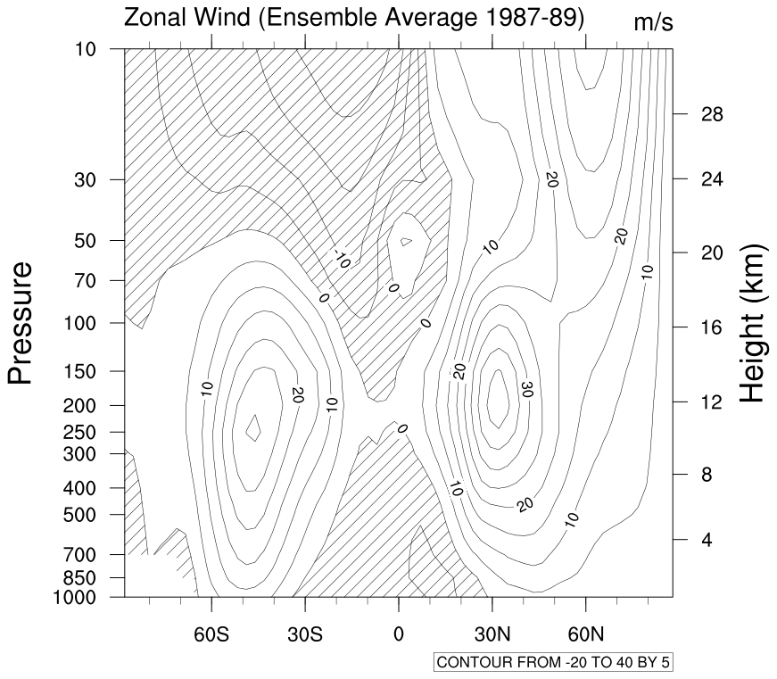h_lat_4.ncl: Shades values less than zero.

ShadeLtContour is the shea utility function that shades regions less than a given number. Note: this function has been superceded by the more versatile gsn_contour_shade. We recommend you use this instead.

There are numerous other contour effects to choose from.

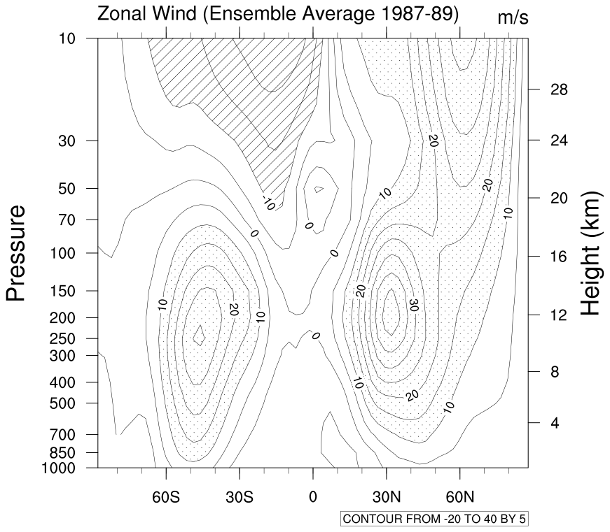h_lat_5.ncl: Shades values less than -10 and stipples greater than +10.

ShadeLtGtContour is the shea utility function that shades regions in a less than/greater than context. Note: this function has been superceded by the more versatile gsn_contour_shade. We recommend you use this instead.

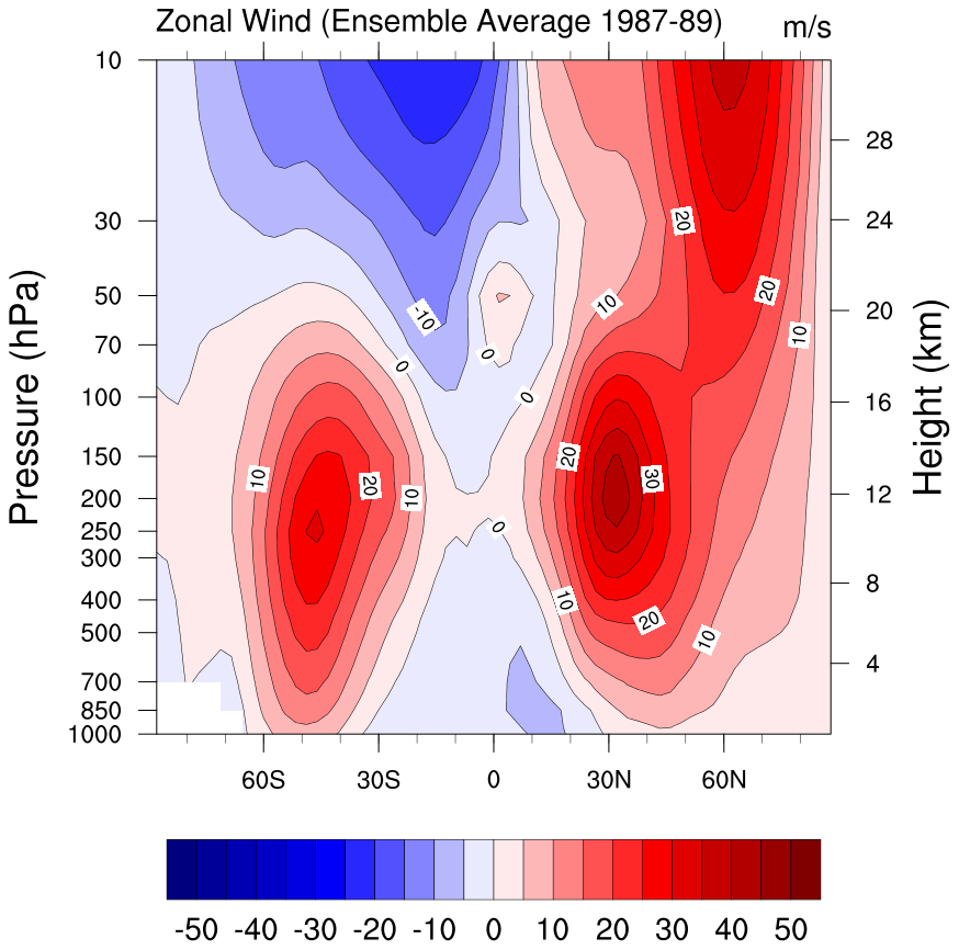
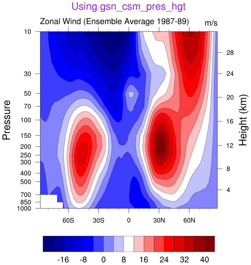
h_lat_6.ncl: Color plot

See the color example page for lots of ways of dealing with color.

A Python version of this projection is available here.

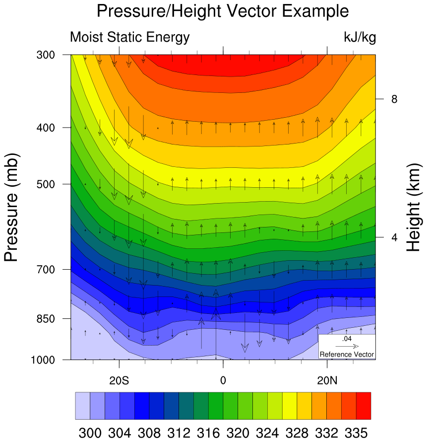h_lat_7.ncl: Example of a vector pressure/height plot.

vcRefAnnoOrthogonalPosF = -0.165, Moves the reference vector orthogonal from its default position.

gsn_csm_pres_hgt_vector is the plot interface that draws vectors over a pressure height plot. Note that vcMapDirection must be set to False in order for the vectors to be pointing in the right direction. In V6.2.0, this resource will be set to False by default for the gsn_csm_pres_hgt_vector function.

Note, in this example, V is set to zero so that only the vertical velocities are plotted. Additionally, the units of omega (mb/day) and v (m/s) have different units. No scaling is used in this example but the user may wish do do so.

h_lat_8.ncl: Demonstrates how to remove the labels on the right axis. These are special labels, so the method is different from removing the left axis labels.

tmYRMode = "Automatic", will override the plot template's explicit setting of the height labels on the right axis.

h_lat_9.ncl: The first part of this script shows a basic pressure-height plot created with gsn_csm_pres_hgt. The second part of the script shows how to recreate this plot from scratch, by overlaying a contour plot on a "LogLin" object.

The point of this script is to allow you more control over the look of pressure-height plot, for example, if you want to change the labels on the right Y axis.

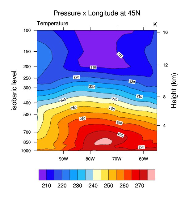
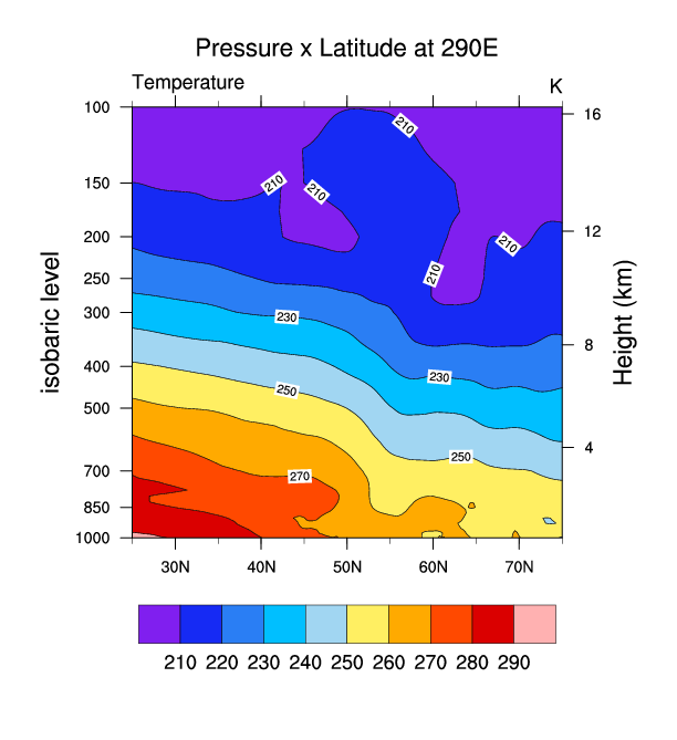
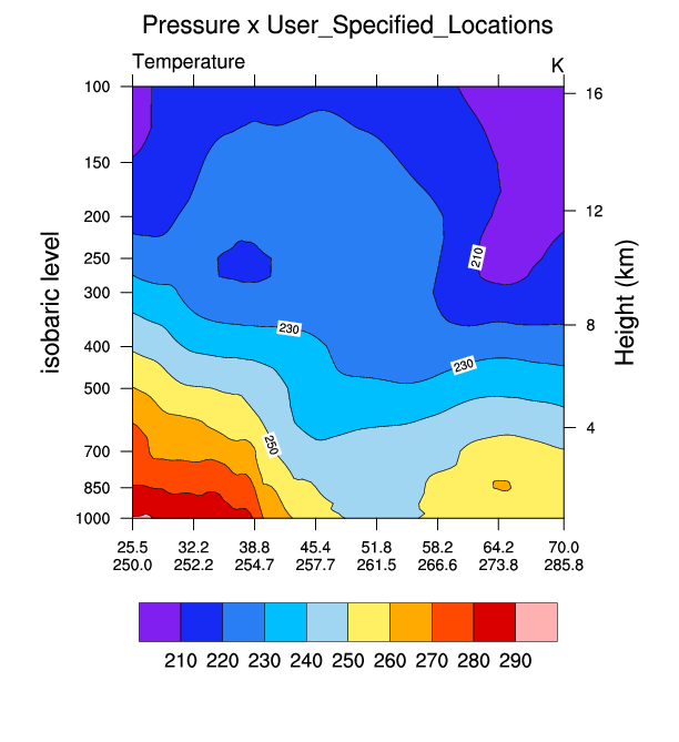narr_5.ncl: This script uses an ESMF generated weight file (See: ESMF Example 30) to efficiently regrid a source NARR curvilinear grid to a rectilinear grid. Then three cross sections are plotted: (a) pressure x longitude; (b) pressure x latitude; and, (c) pressure x user_speciied_set_of_points. For this example the user specified latitude/longitude locations lie along a great circle path between two user specified locations (See: gc_latlon). They could be latitude/longitude locations along a (say) cold front.

ESMF Example 30 was run twice: bilinear and conservative interpolation. Bilinear interpolation would generally be appropriate for any reasonably smooth variable. Conservation interpolation would be recommended for interpolating flux quantities and variables that can be fractal (eg precipitation).

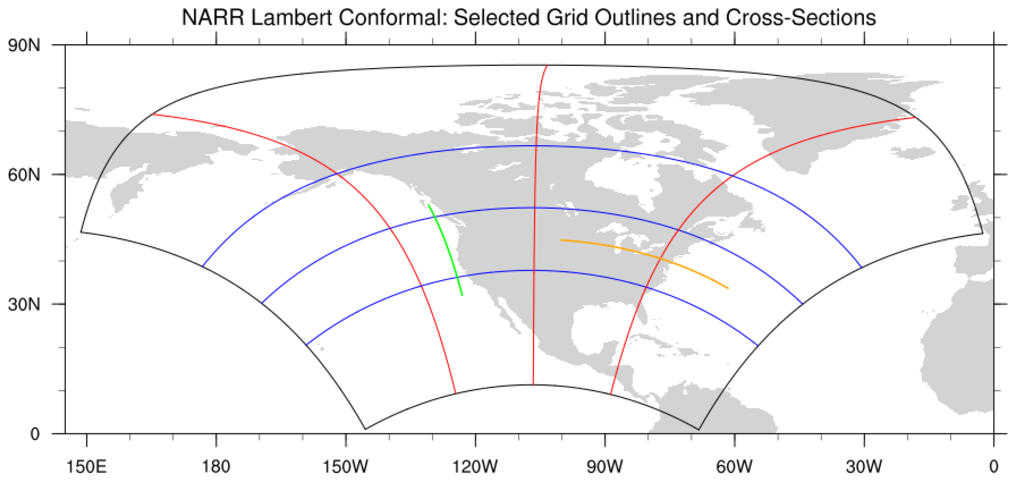
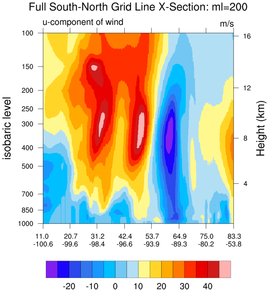
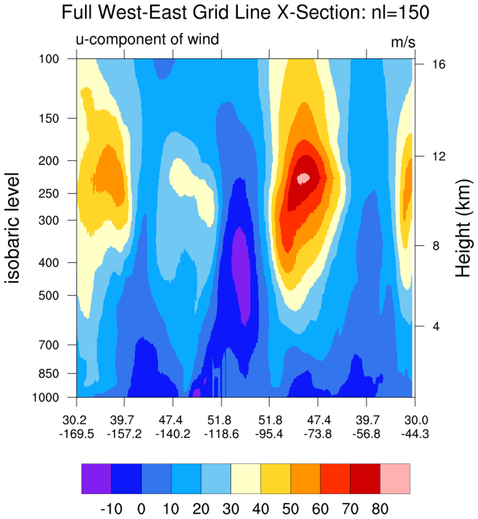
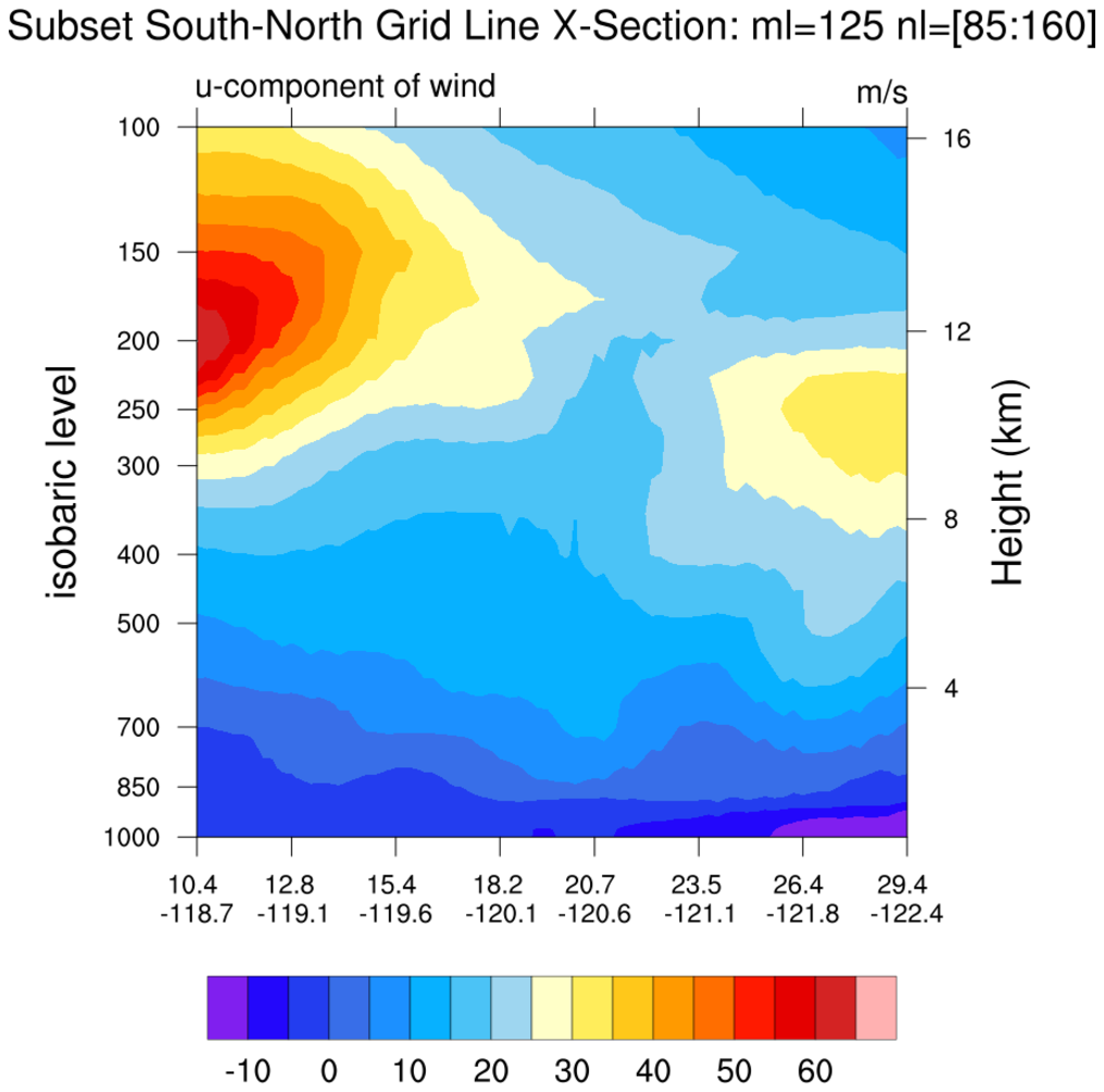
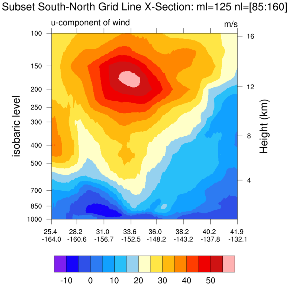narr_6.ncl: The NARR grid is curvilinear. This means that the grid point locations require two-dimensional latitude and longitude arrays. The leftmost figure shows the north, south, west and east boundaries (black outline); selected east-west grid lines (blue); selected north-south grid lines (red); and, user specified subsets of grid lines. Sample 'grid line following' cross sections are created.