NCL Home>
Application examples>
Data Analysis ||
Data files for some examples
 ESMF_regrid_1.ncl /
ESMF_wgts_1.ncl /
ESMF_all_1.ncl:
ESMF_regrid_1.ncl /
ESMF_wgts_1.ncl /
ESMF_all_1.ncl:
 ESMF_regrid_2.ncl /
ESMF_wgts_2.ncl /
ESMF_all_2.ncl:
ESMF_regrid_2.ncl /
ESMF_wgts_2.ncl /
ESMF_all_2.ncl:

 ESMF_regrid_3.ncl /
ESMF_wgts_3.ncl /
ESMF_all_3.ncl:
ESMF_regrid_3.ncl /
ESMF_wgts_3.ncl /
ESMF_all_3.ncl:
 ESMF_regrid_4.ncl /
ESMF_wgts_4.ncl /
ESMF_all_4.ncl:
ESMF_regrid_4.ncl /
ESMF_wgts_4.ncl /
ESMF_all_4.ncl:
 ESMF_regrid_5.ncl /
ESMF_wgts_5.ncl /
ESMF_all_5.ncl:
ESMF_regrid_5.ncl /
ESMF_wgts_5.ncl /
ESMF_all_5.ncl:

 ESMF_regrid_6.ncl /
ESMF_wgts_6.ncl /
ESMF_all_6.ncl:
ESMF_regrid_6.ncl /
ESMF_wgts_6.ncl /
ESMF_all_6.ncl:
 ESMF_regrid_7.ncl /
ESMF_wgts_7.ncl /
ESMF_all_7.ncl:
ESMF_regrid_7.ncl /
ESMF_wgts_7.ncl /
ESMF_all_7.ncl:
 ESMF_regrid_8.ncl /
ESMF_wgts_8.ncl /
ESMF_all_8.ncl /
ESMF_regrid_zoomed_8.ncl:
ESMF_regrid_8.ncl /
ESMF_wgts_8.ncl /
ESMF_all_8.ncl /
ESMF_regrid_zoomed_8.ncl:
 ESMF_regrid_9.ncl /
ESMF_all_9.ncl:
ESMF_regrid_9.ncl /
ESMF_all_9.ncl:
 ESMF_regrid_10.ncl /
ESMF_wgts_10.ncl /
ESMF_all_10.ncl /
ESMF_regrid_neareststod_10.ncl:
ESMF_regrid_10.ncl /
ESMF_wgts_10.ncl /
ESMF_all_10.ncl /
ESMF_regrid_neareststod_10.ncl:
 ESMF_regrid_11.ncl /
ESMF_wgts_11.ncl /
ESMF_all_11.ncl:
ESMF_regrid_11.ncl /
ESMF_wgts_11.ncl /
ESMF_all_11.ncl:
 ESMF_regrid_12.ncl /
ESMF_wgts_12.ncl /
ESMF_regrid_12.ncl /
ESMF_wgts_12.ncl /
ESMF_all_conserve_12.ncl: ESMF_all_patch_12.ncl:
 ESMF_regrid_13.ncl /
ESMF_regrid_unstruct_13.ncl /
ESMF_wgts_13.ncl /
ESMF_all_13.ncl:
ESMF_regrid_13.ncl /
ESMF_regrid_unstruct_13.ncl /
ESMF_wgts_13.ncl /
ESMF_all_13.ncl:
 ESMF_regrid_14.ncl /
ESMF_wgts_14.ncl /
ESMF_all_14.ncl:
ESMF_regrid_14.ncl /
ESMF_wgts_14.ncl /
ESMF_all_14.ncl:


 ESMF_regrid_15.ncl /
ESMF_wgts_15.ncl /
ESMF_all_15.ncl:
ESMF_regrid_15.ncl /
ESMF_wgts_15.ncl /
ESMF_all_15.ncl:
 ESMF_regrid_16.ncl:
 ESMF_regrid_17.ncl /
ESMF_wgts_17.ncl:
ESMF_regrid_17.ncl /
ESMF_wgts_17.ncl:
 ESMF_regrid_18.ncl:
 ESMF_regrid_19.ncl:
 ESMF_regrid_20.ncl:
 ESMF_regrid_21.ncl:
 ESMF_regrid_22.ncl:
 ESMF_regrid_23.ncl: This
example was taken from the HDF examples
page. It shows how to regrid data from a 9 km MODIS Aqua Level-3
HDF4 file to a 0.5 degree grid. The file attributes contain the
geographical information, which is used to generate coordinate
variables for the source grid.
ESMF_regrid_23.ncl: This
example was taken from the HDF examples
page. It shows how to regrid data from a 9 km MODIS Aqua Level-3
HDF4 file to a 0.5 degree grid. The file attributes contain the
geographical information, which is used to generate coordinate
variables for the source grid.

 ESMF_regrid_24.ncl: This
example shows how to regrid data from a POP curvilinear gx1v3 grid
(384 x 320) to a 1.0 degree world grid. It plots sea water potential
temperature on the new grid.
ESMF_regrid_24.ncl: This
example shows how to regrid data from a POP curvilinear gx1v3 grid
(384 x 320) to a 1.0 degree world grid. It plots sea water potential
temperature on the new grid.
 ESMF_regrid_25.ncl /
ESMF_wgts_25.ncl: This
example shows how to regrid CLM data on the 'ne30' to a finite volume grid.
ESMF_regrid_25.ncl /
ESMF_wgts_25.ncl: This
example shows how to regrid CLM data on the 'ne30' to a finite volume grid.
 ESMF_regrid_26.ncl:
This shows how to regrid a ROMS model output to a rectilinear grid.
The ROMS grid information and the model variable output are
contained on separate files.
This specific version of ROMS is for the "Coral configuration."
The original grid has 5km spacing. The rectilinear grid is set to 0.05
degree spacing which corresponds to approximately 5km (~0.05*111km).
ESMF_regrid_26.ncl:
This shows how to regrid a ROMS model output to a rectilinear grid.
The ROMS grid information and the model variable output are
contained on separate files.
This specific version of ROMS is for the "Coral configuration."
The original grid has 5km spacing. The rectilinear grid is set to 0.05
degree spacing which corresponds to approximately 5km (~0.05*111km).
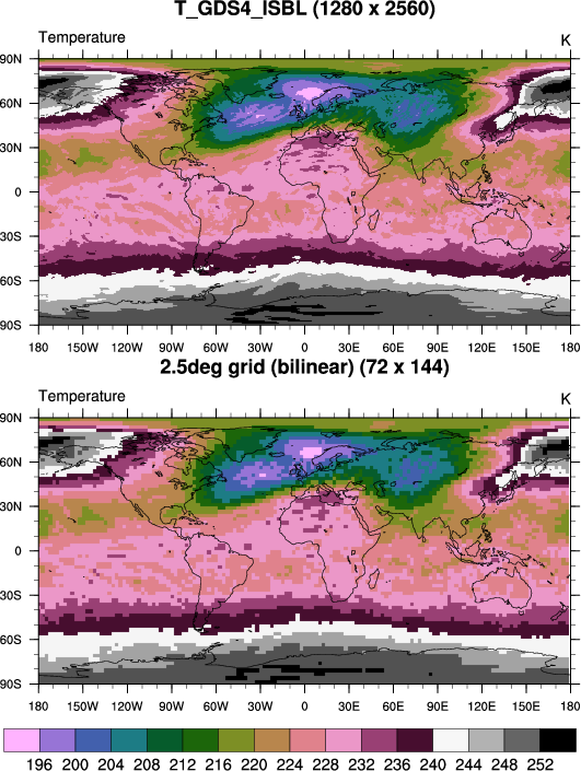
 ESMF_regrid_27.ncl:
This example shows how to regrid variables from a suite of ECMWF files
that contain an Operational Model Analysis grid with a 1280 x 2560
regular Gaussian grid to a lower resolution 2.5 degree grid.
ESMF_regrid_27.ncl:
This example shows how to regrid variables from a suite of ECMWF files
that contain an Operational Model Analysis grid with a 1280 x 2560
regular Gaussian grid to a lower resolution 2.5 degree grid.
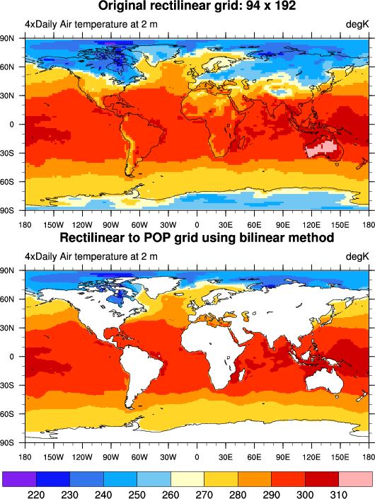
 ESMF_regrid_28.ncl:
The demonstrates how to regrid variables on a rectilinear grid onto
a POP curvilinear grid. The source variable is type short and
must be unpacked prior to regridding. Further, only the 1st time
step is read because only the spatial information (latitudes
and longitudes) is needed for weight generation. POP variables have no values
over land. Hence, a variable from the target POP file is read
and used to generate a mask.
ESMF_regrid_28.ncl:
The demonstrates how to regrid variables on a rectilinear grid onto
a POP curvilinear grid. The source variable is type short and
must be unpacked prior to regridding. Further, only the 1st time
step is read because only the spatial information (latitudes
and longitudes) is needed for weight generation. POP variables have no values
over land. Hence, a variable from the target POP file is read
and used to generate a mask.
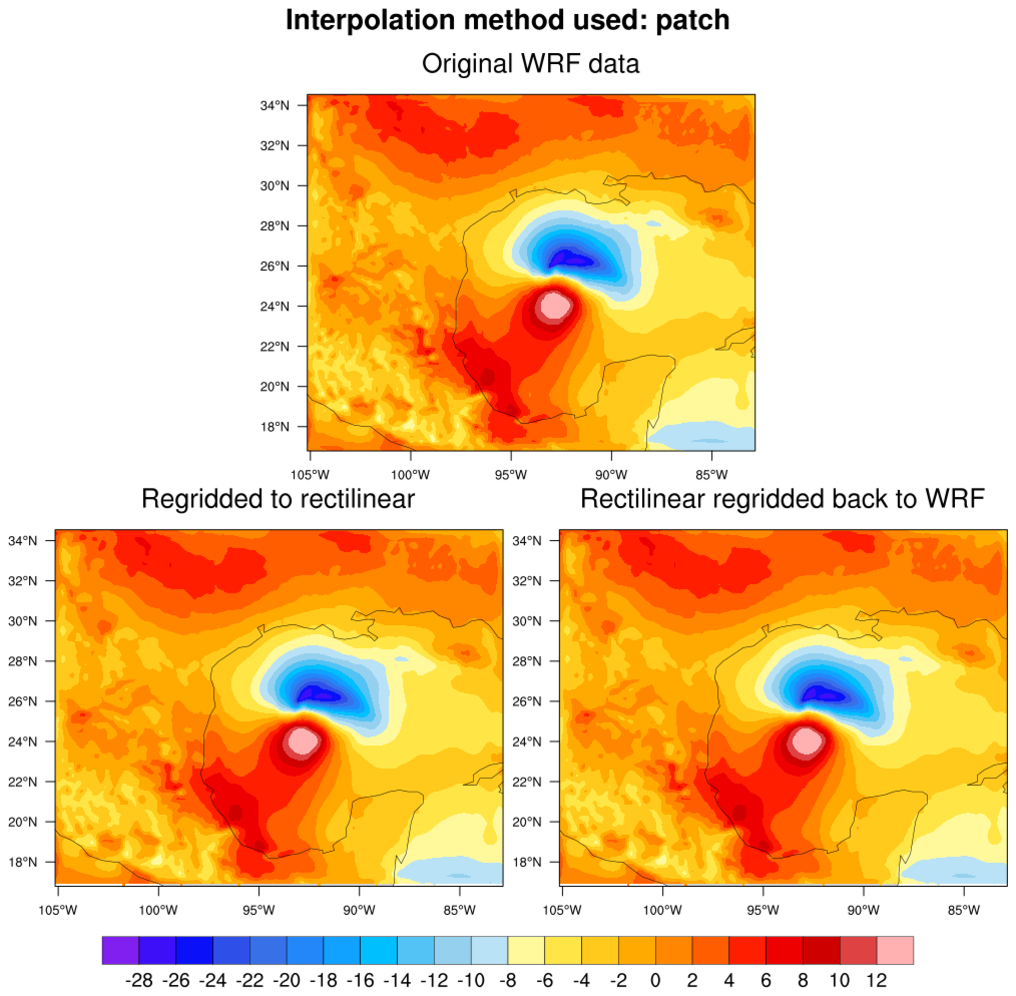
 ESMF_regrid_29.ncl /
ESMF_wgts_29.ncl:
These scripts show how you can use a two-step process to regrid WRF data.
ESMF_regrid_29.ncl /
ESMF_wgts_29.ncl:
These scripts show how you can use a two-step process to regrid WRF data.

 ESMF_wgts_30.ncl:
This script regrids a NARR grid which is a curvilinear grid to a 0.25 rectilinear grid (Part A).
Then for illustration it regrids the rectilinear grid back to the original NARR grid (Part B).
The rectilinear->NARR section (Part B) could easily be extracted and used as a template to regrid any
rectilinear grid to the NARR grid.
ESMF_wgts_30.ncl:
This script regrids a NARR grid which is a curvilinear grid to a 0.25 rectilinear grid (Part A).
Then for illustration it regrids the rectilinear grid back to the original NARR grid (Part B).
The rectilinear->NARR section (Part B) could easily be extracted and used as a template to regrid any
rectilinear grid to the NARR grid.
 ESMF_regrid_31.ncl:
This script regrids IGBP vegetation categorical data which is on
a high-resolution 1080 x 2160 grid, to a 1 degree lat/lon grid.
ESMF_regrid_31.ncl:
This script regrids IGBP vegetation categorical data which is on
a high-resolution 1080 x 2160 grid, to a 1 degree lat/lon grid.
 ESMF_regrid_32.ncl: This
example regrids WRF output temperature data to both a 1.0 and 0.5 degree
grid, and compares them in a panel plot.
ESMF_regrid_32.ncl: This
example regrids WRF output temperature data to both a 1.0 and 0.5 degree
grid, and compares them in a panel plot.
 ESMF_regrid_33.ncl: This
example regrids the 'gland5.nc' (Greenland Developmental Data Set: Greenland_5km_dev1.1.nc)
data on a very high resolution 5km grid to a 0.5 degree grid using the bilinear, patch and conserve
interpolation methods. A subsequent run generated a separate regrid weight file for a 1x1 resolution.
See: gland_2/3
for application of these weight files.
ESMF_regrid_33.ncl: This
example regrids the 'gland5.nc' (Greenland Developmental Data Set: Greenland_5km_dev1.1.nc)
data on a very high resolution 5km grid to a 0.5 degree grid using the bilinear, patch and conserve
interpolation methods. A subsequent run generated a separate regrid weight file for a 1x1 resolution.
See: gland_2/3
for application of these weight files.
 ESMF_regrid_34.ncl:
This interpolates data on a NARR grid to a WRF grid. Here, the WRF grid covers a much smaller area than the source NARR grid. This is a curvilinear to curvilinear interpolation.
ESMF_regrid_34.ncl:
This interpolates data on a NARR grid to a WRF grid. Here, the WRF grid covers a much smaller area than the source NARR grid. This is a curvilinear to curvilinear interpolation.
 ESMF_regrid_35.ncl:
Using the ESMF 'bilinear', 'patch' and 'conserve' methods to interpolate a high-resolution
(0.1x0.1) rectilinear regional grid a lower resolution (1x1) rectilinear grid.
This is similar to several
other ESMF examples. However, the source data is a 'bit fractal' in nature. It illustrates
the results of the three methods.
ESMF_regrid_35.ncl:
Using the ESMF 'bilinear', 'patch' and 'conserve' methods to interpolate a high-resolution
(0.1x0.1) rectilinear regional grid a lower resolution (1x1) rectilinear grid.
This is similar to several
other ESMF examples. However, the source data is a 'bit fractal' in nature. It illustrates
the results of the three methods.
 ESMF_regrid_36.ncl:
Interpolate data from a high resolution (0.1x0.1 [1800x3600]) global grid
to a regional curvilinear (WRF) grid using 'bilinear', 'patch', 'nearestod',
and 'conserve' methods. NCL's
coordinate
subscripting is used to extract an area subset surrounding China. This reduces the
interpolation time.
ESMF_regrid_36.ncl:
Interpolate data from a high resolution (0.1x0.1 [1800x3600]) global grid
to a regional curvilinear (WRF) grid using 'bilinear', 'patch', 'nearestod',
and 'conserve' methods. NCL's
coordinate
subscripting is used to extract an area subset surrounding China. This reduces the
interpolation time.
 ESMF_regrid_37.ncl:
The is similar to the ESMF_wgts_29.ncl script. It regrids the WRF's zonal
and meridional wind components onto a rectilinear grid. It then uses
the uv2dv_cfd function to compute divergence on the rectilinear
grid and then regrids the divergence back onto the original WRF grid.
ESMF_regrid_37.ncl:
The is similar to the ESMF_wgts_29.ncl script. It regrids the WRF's zonal
and meridional wind components onto a rectilinear grid. It then uses
the uv2dv_cfd function to compute divergence on the rectilinear
grid and then regrids the divergence back onto the original WRF grid.
Example pages containing: tips | resources | functions/procedures
NCL: Regridding using NCL with Earth System Modeling Framework (ESMF) software
For a general overview on regridding, see the
"Regridding
Overview" section in
the Climate Data
Guide.
Quick note: if the examples on this page are not
helpful, visit NCL templates page
for a list of generic ESMF regridding template scripts.
This page shows how you can use ESMF regridding functions to
regrid data on
rectilinear,
curvilinear, and
unstructured
"source" grids, to "destination" grids of any of these types.
ESMF regridding creates a weights file that you can use to
regrid other variables on the same grid. See
the special note below
about weights and missing values.
This software is only available in NCL version 6.1.0 and later.
The Earth System Modeling Framework (ESMF) is "software for building and coupling weather, climate, and related models". The ESMF "ESMF_RegridWeightGen" tool has been incorporated into NCL for generating weights for interpolating (regridding) data from a one grid to another.
Many thanks go to Robert Oehmke of NOAA---one of the developers of ESMF---for his consulting and patience in helping us learn and incorporate this software. Many thanks also go to Mohammad Abouali, who developed the original version of these NCL functions as part of a CISL SIParCS summer internship program.
The basic steps of NCL/ESMF regridding involve:
- Reading or generating the "source" grid.
- Reading or generating the "destination" grid.
- Creating special NetCDF files that describe these two grids.
- *Generating a NetCDF file that contains the weights.
- Applying the weights to data on the source grid, to interpolate the data to the destination grid.
- Copying over any metadata to the newly regridded data.
*This is the most important step. Once you have a weights file, you can skip steps #1-4 if you are interpolating data on the same grids.
ESMF regridding in NCL can be done one of three ways; each method has its advantages:
- Via a single call to the function
ESMF_regrid - this method does most
of all of the above steps for you, but can be redundant if you
are generating the same weights file over and over.
- Via a call to the function
ESMF_regrid_with_weights - this
method is straight-forward and faster; it requires that you already
have the weights file. You can use the weights file generated
from an initial call to ESMF_regrid,
or from the third method described below.
- Via a multi-step process - this method is the most complicated,
but allows for individual control over all the regridding steps. This
method is not really recommended, unless you understand the multi-step
regridding process well. See the detailed
description below.
Several of the examples below include more than one script showing you the various methods:
- Method 1: ESMF_regrid_n.ncl
- Method 2: ESMF_wgts_regrid_n.ncl
- Method 3: ESMF_all_n.ncl
More detailed description of ESMF regridding
For the special NetCDF files that are generated to describe the source and destination grids: SCRIP (Spherical Coordinate Remapping and Interpolation Package) is used to describe the rectilinear and curvilinear grids, and an internal ESMF format is used to describe the unstructured grids.
When the weights file is generated, there are five types of interpolation methods supported by ESMF software:
- "bilinear" - the algorithm used by this application to generate
the bilinear weights is the standard one found in many textbooks. Each
destination point is mapped to a location in the source mesh, the
position of the destination point relative to the source points
surrounding it is used to calculate the interpolation weights.
- "patch" - this method is the ESMF version of a technique called
"patch recovery" commonly used in finite element modeling. It
typically results in better approximations to values and derivatives
when compared to bilinear interpolation.
- "conserve" - this method will typically have a larger
interpolation error than the previous two methods, but will do a much
better job of preserving the value of the integral of data between the
source and destination grid.
The "conserve" method requires that the corners of the lat/lon grid be input. NCL will try to provide a guess at the corners if you don't provide them, but this could likely result in failure.
You can (and are highly recommended to) provide your own grid corners via the special Src/Dst/GridCornerLat/Lon resources. They must be provided as an N x 4 array, where N represents the dimensionality of the center lat/lon grid. For example, if the center lat/lon grid is dimensioned 256 x 220, then the corner arrays must be 256 x 220 x 4. Sometimes the corner grids are provided on the file along with the center grids, with names like "lat_vertices"/"lon_vertices" or "lat_bounds"/"lon_bounds".
- "neareststod" / "nearestdtos" - Available in version 6.2.0 and later. The nearest neighbor methods work by associating a point in one set with the closest point in another set. If two points are equally close then the point with the smallest index is arbitrarily used (i.e. the point with that would have the smallest index in the weight matrix). There are two versions of this type of interpolation available in the regrid weight generation application. One of these is the nearest source to destination method ("neareststod"). In this method each destination point is mapped to the closest source point. The other of these is the nearest destination to source method ("nearestdtos"). In this method each source point is mapped to the closest destination point. Note, that with this method the unmapped destination point detection doesn't work, so no error will be returned even if there destination points which don't map to any source point.
Special note about weights files and missing values:
You can use the same weights file to regrid across other levels and timesteps of the same variable, or across other variables, as long as the lat/lon grid that you are regridding from and to are exactly the same, and, if you use the special SrcMask2D/DstMask2D/Mask2D options, that your masks are exactly the same. The masks are 2D arrays filled with 0's and 1's that indicate where your data values and/or lat/lon values are missing. Here's a description from Robert Oehmke of ESMF about this:
What the mask does is remove the entity (cell or point depending on the type of regridding) from consideration by the regridder. If it's a source cell then no destination entities are mapped to it. If it's a destination entity, then it's not interpolated to. There is a little more in-depth discussion in the ESMF reference manual.
Right now, masking needs to be done before weight calculation so the regridding knows what it should ignore, so if the mask changes then you need to regenerate weights. We actually have a feature request ticket for handling this type of missing value situation more fluidly. The plan is to have the interpolation automatically not use missing values when they are encountered in a data field. Which would allow the same weights to be used for all the levels.
One trick you can do right now with missing values and a weight file is to do two interpolations to tell you where the missing values will spread in the destination field. First interpolate a field containing all 0's except for where the missing values are set the missing value locations to 1, the result of this interpolation tells you which destination locations (the ones whose values >0.0) will be affected by the missing values, so you can ignore them after interpolating the data. (You could also do something like this in one step during the data interpolation if you have a restricted range for your data and you use a value way outside that range for your missing value.) This, of course, will give you a coarser result than using the masking, but will probably be more efficient than recalculating the weights each time.
Detailed description of the multi-step regridding process (method #3)
- Write the description of the source grid to an intermediate SCRIP
or ESMF file using one of the following functions:
- Write the description of the destination grid to an intermediate
SCRIP or ESMF file using the same functions as above.
- Generate the weights file
using ESMF_regrid_gen_weights.
[The weights are generated internally using the offline ESMF regridding tool called "ESMF_RegridWeightGen". This weight file can be reused for other variables with the same source and destination grids, enabling you to skip steps #1-3.]
- Interpolate the data from the source grid to the destination grid using ESMF_regrid_with_weights.
Regrid and create netCDF files containing regridded variables
Most of the following examples show: (a) how to generate the weights needed to regrid variables; (b) apply the weights to a variable and (c) generate a plot showing the original and regridded variable.
Another approach is to regrid all or selected variables and then save the regridded data to a netCDF file for later use. In NCL, there are two methods that can be used to generate netCDF files. The following scripts, which operate on the CAM SE grid (See Example 25), illustrate how to save the regridded data via methods 1 and 2. The latter is considerably more complicated because it uses two steps to create the netCDF. However, the advantage is that it is the more efficient way to generate the netCDF file. The first step is to predefine the contents of the output file. No data values are written during this step. The second step is to regrid each variable and then write the regridded values into the predefined file structure.
             Method 1: se2fv_esmf.regrid2file.ncl
             Method 2: se2fv_esmf.regrid2file.ncl_predefine
Many of the examples below are being updated to include examples of
writing results to NetCDF files. See
examples 1, 2,
and 27.
 ESMF_regrid_1.ncl /
ESMF_wgts_1.ncl /
ESMF_all_1.ncl:
ESMF_regrid_1.ncl /
ESMF_wgts_1.ncl /
ESMF_all_1.ncl:
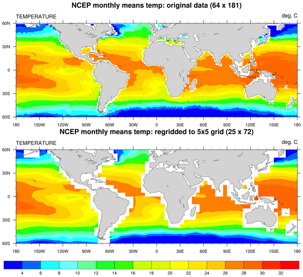
This example shows how to to regrid data on a global NCEP rectilinear grid (64 x 181) to a 5x5 degree lat/lon grid (25 x 72), using the "bilinear" interpolation method. The NCEP file, "sst.nc", can be found on our data page.
The regridded results are written to a new NetCDF file using the "easy" but inefficient method.
The original data contains missing values, so it's important to set the special SrcMask2D option to indicate where the missing values are. For more information on weights files and masking, see the special note above.
The three scripts produce identical results:
- ESMF_all_1.ncl - does the regridding in several steps
- ESMF_regrid_1.ncl - does the regridding in a single call to ESMF_regrid
- ESMF_wgts_1.ncl - uses an existing weights file and does the regridding with a call to ESMF_regrid_with_weights
This example was taken from the "regrid_1.ncl" example on the original regridding examples page, which uses the linint2 function to do the regridding.
 ESMF_regrid_2.ncl /
ESMF_wgts_2.ncl /
ESMF_all_2.ncl:
ESMF_regrid_2.ncl /
ESMF_wgts_2.ncl /
ESMF_all_2.ncl:
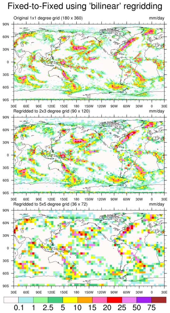
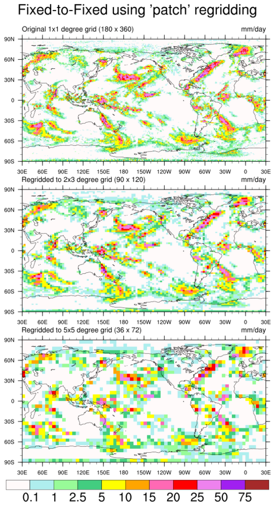
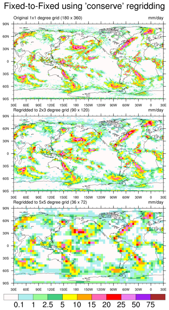
This example shows how to regrid from a 1x1 degree global rectilinear grid (180 x 360) to lower resolution 2x3 degree (90 x 120) and 5x5 degree grid (36 x 72), using three interpolation methods: bilinear, patch, and conserve.
The regridded results are written to separate NetCDF files using the "easy" but inefficient method.
This example was taken from the "regrid_6.ncl" example on the original regridding examples page, which uses the area_conserve_remap_Wrap function to do the regridding.
ESMF_regrid_2.ncl does the regridding in a single call to ESMF_regrid.

 ESMF_regrid_3.ncl /
ESMF_wgts_3.ncl /
ESMF_all_3.ncl:
ESMF_regrid_3.ncl /
ESMF_wgts_3.ncl /
ESMF_all_3.ncl:
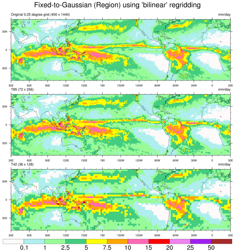
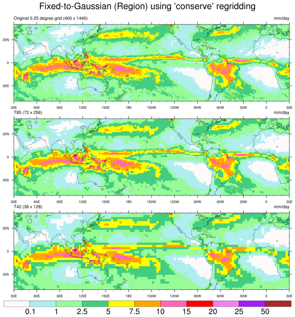
This example shows how to regrid from a 0.25 degree global grid (400 x 1440) to a T42 (36 x 128) and T85 grid (72 x 256), using three interpolation methods: bilinear, patch, and conserve.
This example was taken from the "regrid_11.ncl" example on the original regridding examples page, which uses the area_conserve_remap_Wrap function to do the regridding.
ESMF_regrid_3.ncl does the regridding in a single call to ESMF_regrid.
 ESMF_regrid_4.ncl /
ESMF_wgts_4.ncl /
ESMF_all_4.ncl:
ESMF_regrid_4.ncl /
ESMF_wgts_4.ncl /
ESMF_all_4.ncl:
This example shows how to regrid from a subset (511 x 1081) of a high-resolution rectilinear global elevation grid (5401 x 10801) to a low-resolution 0.5 degree regional grid (35 x 73), using the "conserve" interpolation method.
This example was taken from the "regrid_13.ncl" example on the original regridding examples page, which uses the area_conserve_remap_Wrap to do the regridding.
 ESMF_regrid_5.ncl /
ESMF_wgts_5.ncl /
ESMF_all_5.ncl:
ESMF_regrid_5.ncl /
ESMF_wgts_5.ncl /
ESMF_all_5.ncl:
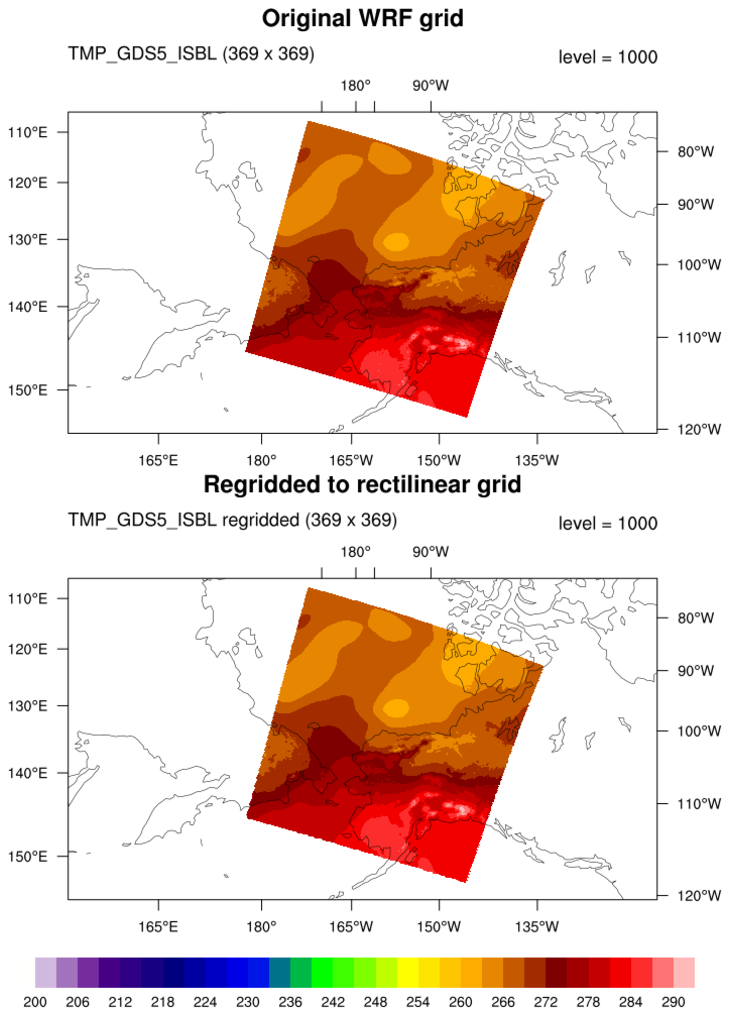
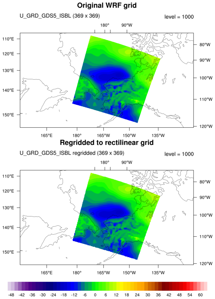
This example shows how to regrid two different datasets from a curvilinear WRF grid to a rectilinear grid of the same size (369 x 369), using the default "bilinear" interpolation method.
The weights are generated just once, and used to regrid two different variables on the file.
The variables plotted have 19 levels, but only the 19th level is plotted. If you want to interpolate and plot all 19 levels, set the LEVEL variable to -1.

 ESMF_regrid_6.ncl /
ESMF_wgts_6.ncl /
ESMF_all_6.ncl:
ESMF_regrid_6.ncl /
ESMF_wgts_6.ncl /
ESMF_all_6.ncl:
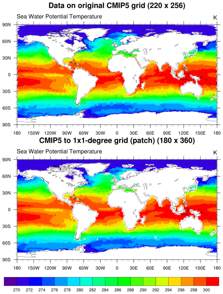
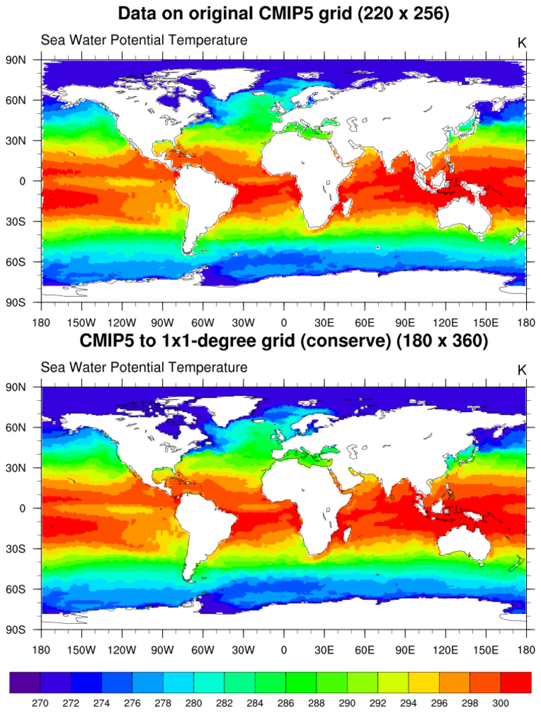
This example shows how to regrid from a curvilinear CMIP5 global grid (220 x 256) to a 1x1 degree grid, using three interpolation methods. Note that the grid corners are needed for the "conserve" method, and they are provided on the file as variables called "lat_vertices" and "lon_vertices". The special attributes "GridCornerLat" and "GridCornerLon" were set to these arrays before calling curvilinear_to_SCRIP.
 ESMF_regrid_7.ncl /
ESMF_wgts_7.ncl /
ESMF_all_7.ncl:
ESMF_regrid_7.ncl /
ESMF_wgts_7.ncl /
ESMF_all_7.ncl:
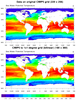
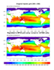
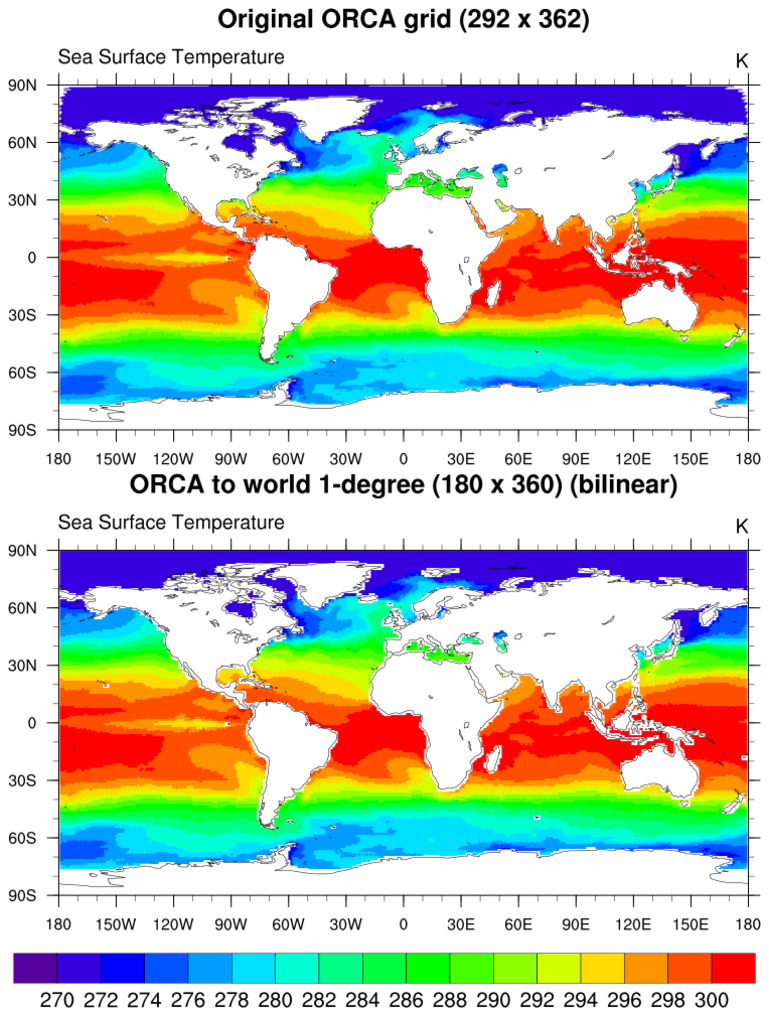
This example shows how to regrid from a curvilinear ORCA global grid (292 x 362) to a 1x1 degree grid, using the default "bilinear" method.
 ESMF_regrid_8.ncl /
ESMF_wgts_8.ncl /
ESMF_all_8.ncl /
ESMF_regrid_zoomed_8.ncl:
ESMF_regrid_8.ncl /
ESMF_wgts_8.ncl /
ESMF_all_8.ncl /
ESMF_regrid_zoomed_8.ncl:
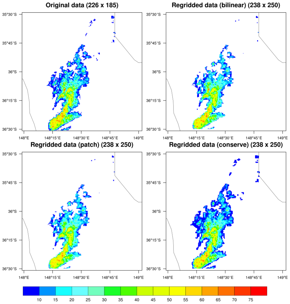
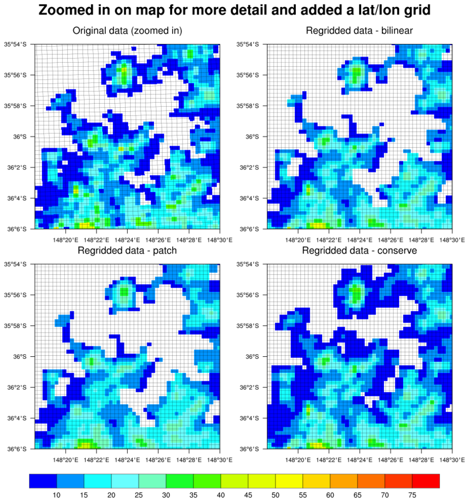
This example shows how to regrid curvilinear regional swath data (265 x 185) to a rectilinear grid (238 x 250) read off a file. Three interpolation methods are compared here.
The ESMF_regrid_zoomed_8.ncl example is similar to ESMF_regrid_8.ncl, except it shows how to zoom in on an area of interest in the map so you can see more detail of the regridding results. The grid lines for both the source grid and destination grids were added with a call to gsn_coordinates.
 ESMF_regrid_9.ncl /
ESMF_all_9.ncl:
ESMF_regrid_9.ncl /
ESMF_all_9.ncl:
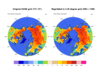
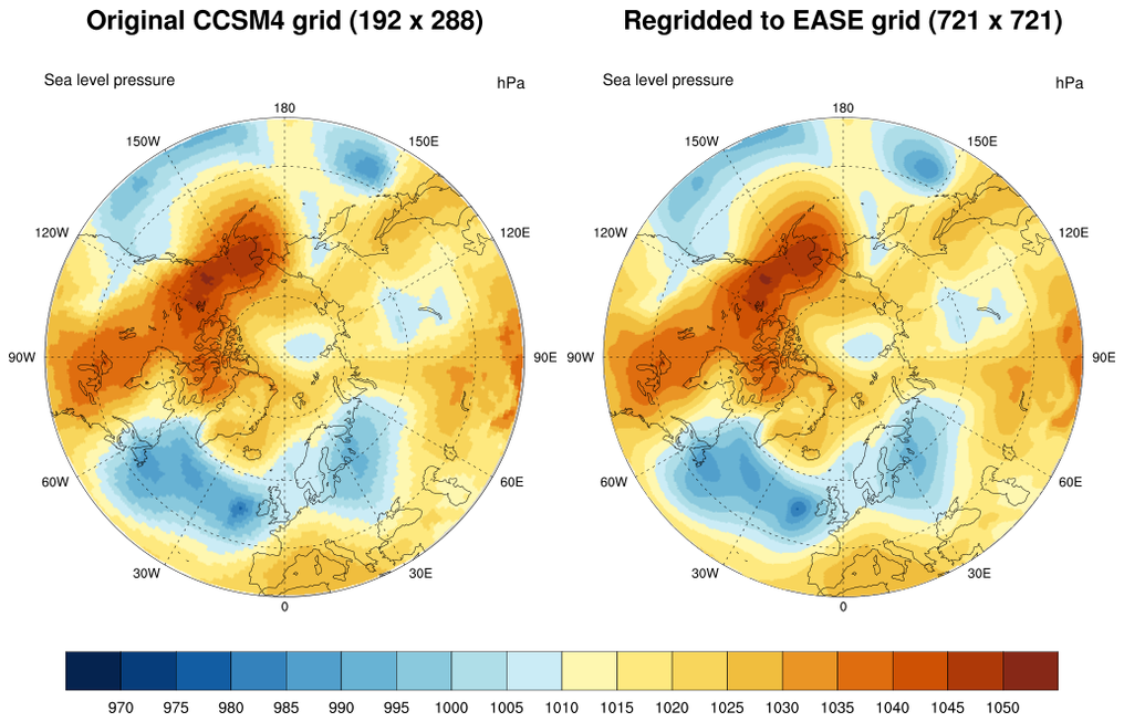
This example hows how to regrid CCSM4 rectilinear data (192 x 288) to a curvilinear EASE grid (721 x 721), using the "patch" method.
This script took 148 CPU seconds on a MacBook Pro, using a single-threaded version of the ESMF_RegridWeightGen tool.
 ESMF_regrid_10.ncl /
ESMF_wgts_10.ncl /
ESMF_all_10.ncl /
ESMF_regrid_neareststod_10.ncl:
ESMF_regrid_10.ncl /
ESMF_wgts_10.ncl /
ESMF_all_10.ncl /
ESMF_regrid_neareststod_10.ncl:
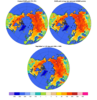
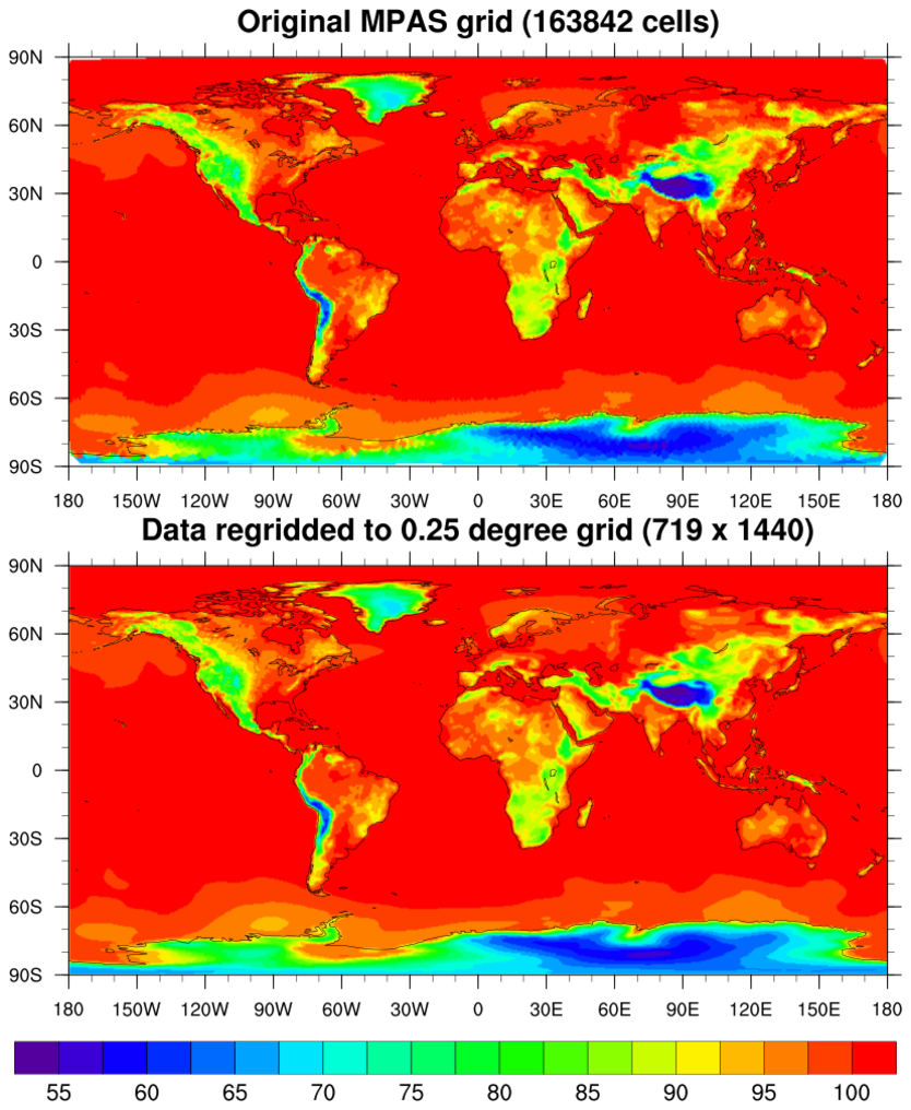
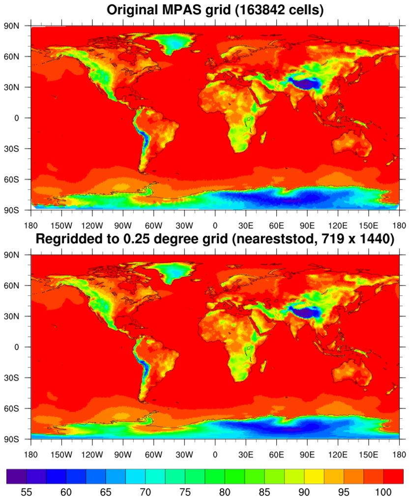
This example shows how to regrid unstructured MPAS data, which is on a hexagonal grid (163842 cells) to a 0.25 degree grid (719 x 440).
The first three scripts use the default "bilinear" method, and the last one uses the nearest neighbor algorithm, added in NCL version 6.2.0 and
 ESMF_regrid_11.ncl /
ESMF_wgts_11.ncl /
ESMF_all_11.ncl:
ESMF_regrid_11.ncl /
ESMF_wgts_11.ncl /
ESMF_all_11.ncl:
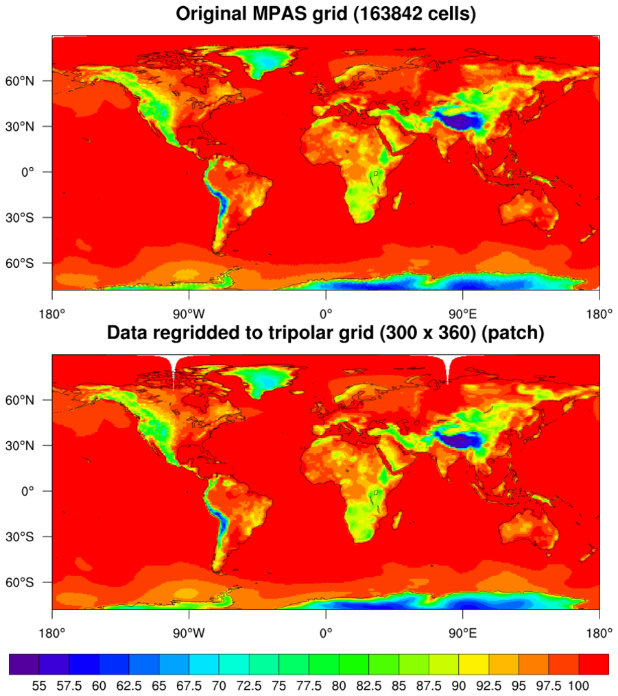
This example uses the same unstructured MPAS data as the previous example, but regrids it to a curvilinear tripolar grid (300 x 360) read off a file. The "patch" interpolation method is used.
 ESMF_regrid_12.ncl /
ESMF_wgts_12.ncl /
ESMF_regrid_12.ncl /
ESMF_wgts_12.ncl /ESMF_all_conserve_12.ncl: ESMF_all_patch_12.ncl:
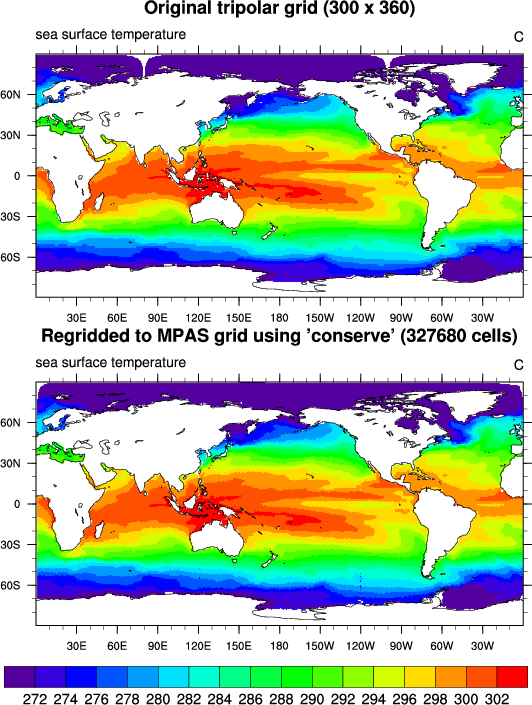
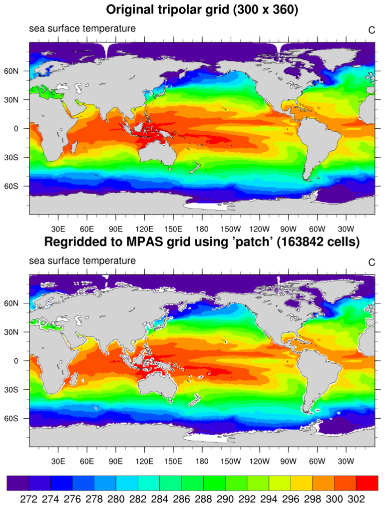
This example is the reverse of the previous example: it regrids data from a curvilinear tripolar grid (300 x 360) to an unstructured MPAS grid (hexagonal grid, 163842 cells). Both the "patch" and "conserve" interpolation methods are used.
The "conserve" method requires the grid corners in addition to the grid centers. If you don't provide the grid corners (via the special "GridCornerLat/GridCornerLon" attributes), then NCL will try to approximate them for you. It's better to provide them if possible.
When you regrid to an unstructured grid, you MUST set Opt@DstGridType = "unstructured" so the ESMF regridding code knows you have an unstructured grid, and not a rectilinear grid that has the same length for its lat/lon arrays.
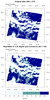
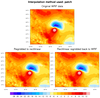
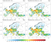
 ESMF_regrid_13.ncl /
ESMF_regrid_unstruct_13.ncl /
ESMF_wgts_13.ncl /
ESMF_all_13.ncl:
ESMF_regrid_13.ncl /
ESMF_regrid_unstruct_13.ncl /
ESMF_wgts_13.ncl /
ESMF_all_13.ncl:
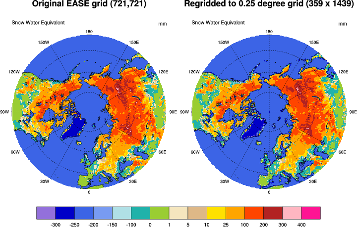
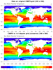
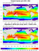
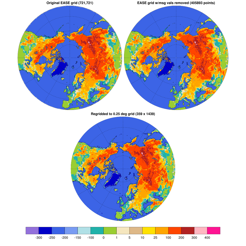
This example regrids data from a curvilinear EASE grid (721 x 721) to a 0.25 degree global grid (359 x 1439). The "patch" interpolation method is used.
The EASE lat/lon grid contains missing values, so it's important to set the special SrcMask2D option to indicate where the missing values are. For more information on weights files and masking, see the special note above. Note that because there are so many missing values, you will see numerous warnings "Entire input array contains missing values, can't compute average". These can be safely ignored.
To see a version of this script that removes all the missing lat/lon values by turning it into an unstructured grid, see "ESMF_regrid_unstruct_13.ncl". This script will take longer to run, because it has to generate a triangular mesh under the hood. The second image above is the one generated by this script. It shows plots of the data on the original curvilinear grid, the unstructured grid with missing values removed, and regridded to the 0.25 degree grid.
 ESMF_regrid_14.ncl /
ESMF_wgts_14.ncl /
ESMF_all_14.ncl:
ESMF_regrid_14.ncl /
ESMF_wgts_14.ncl /
ESMF_all_14.ncl:
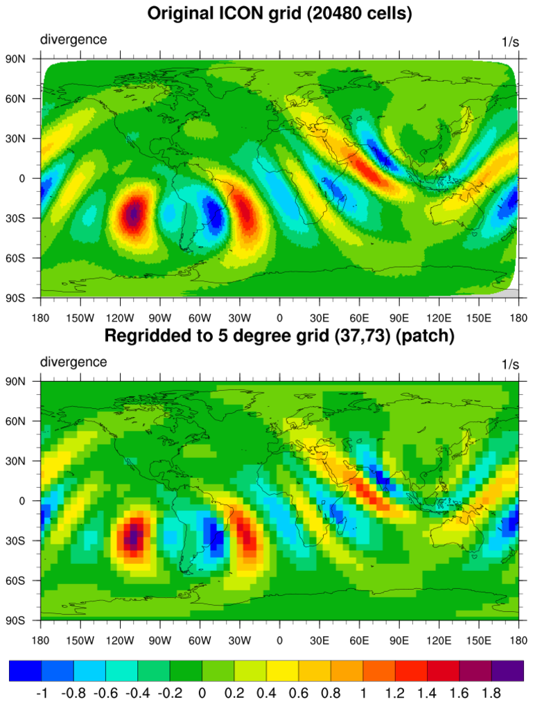
This example regrids triangular mesh (unstructured) data from the ICON model (20480 cells) to a 5 degree grid (37 x 73).
For more examples on plotting ICON data, see the "Visualizing ICON model data" examples page.

 ESMF_regrid_15.ncl /
ESMF_wgts_15.ncl /
ESMF_all_15.ncl:
ESMF_regrid_15.ncl /
ESMF_wgts_15.ncl /
ESMF_all_15.ncl:
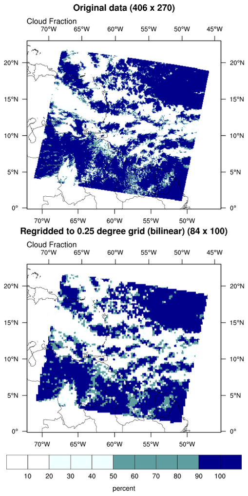
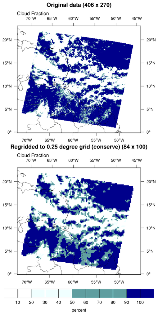
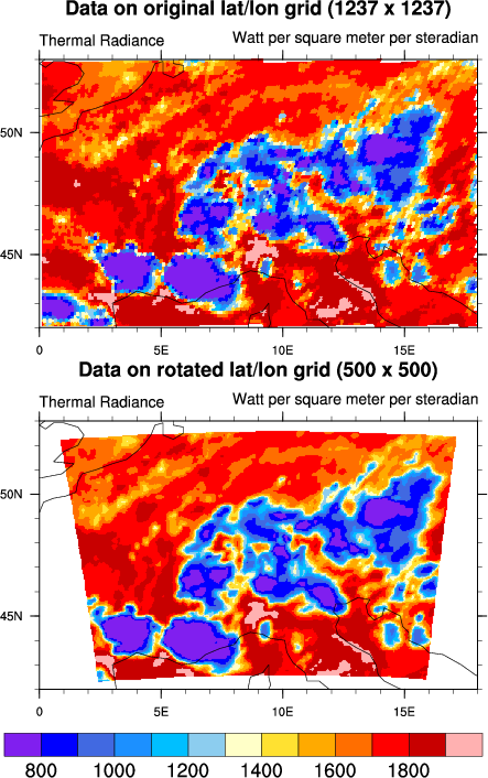
This example shows how to regrid curvilinear regional swath data (406 x 270) to a 0.25 degree regional grid (84 x 100) using three interpolation methods.
 ESMF_regrid_16.ncl:
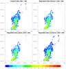
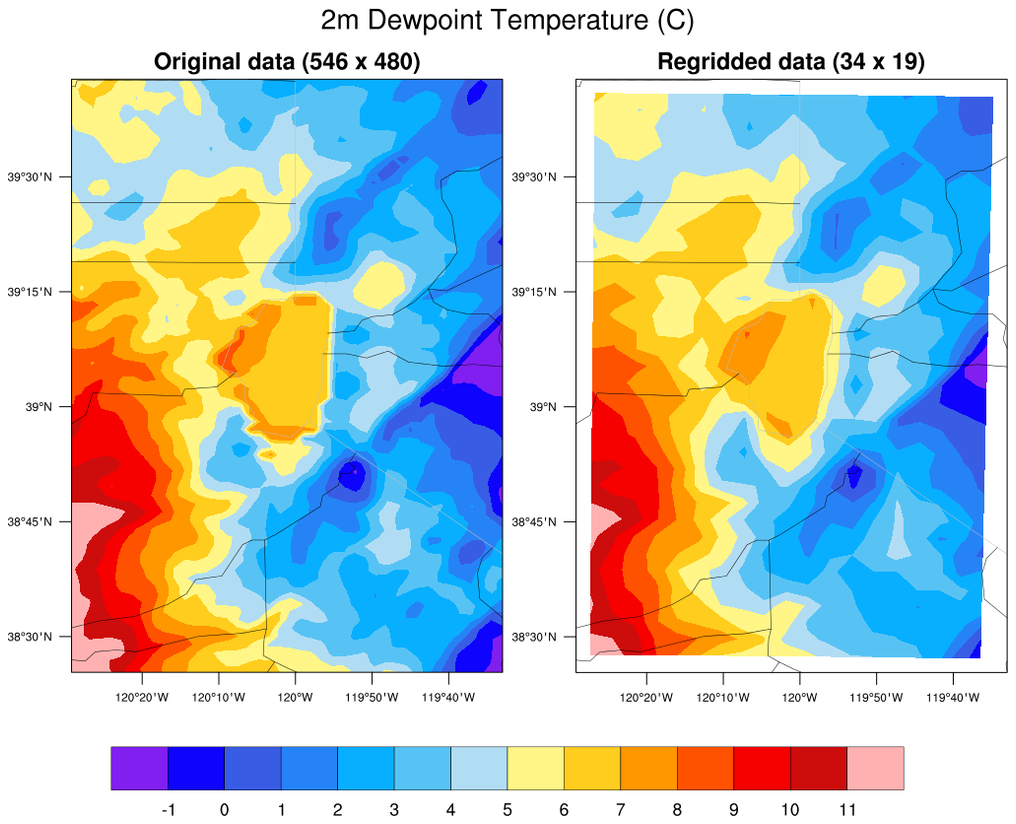
This example shows how to regrid from a WRF curvilinear regional grid (546 x 480) to a much coarser MM5 curvilinear grid (34 x 19) using bilinear interpolation.
The variable regridded is "td2" (2m dewpoint temperature), but you can modify this script to do any 2D or 3D variable on the file. It should also work for more dimensions with slight modification.
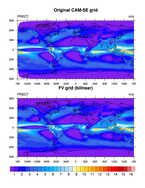 ESMF_regrid_17.ncl /
ESMF_wgts_17.ncl:
ESMF_regrid_17.ncl /
ESMF_wgts_17.ncl:
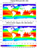
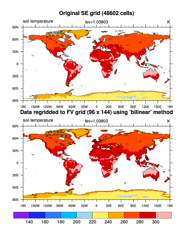
This example shows how to regrid from a CAM-SE (cubed sphere) unstructured grid with 48602 cells to a 96 x 144 finite volume (FV) rectilinear grid.
In this script, if you want to regrid to a subregion of the FV grid, then set SUBREGION to True, and set minlat/maxlat/minlon/maxlon to the desired region.
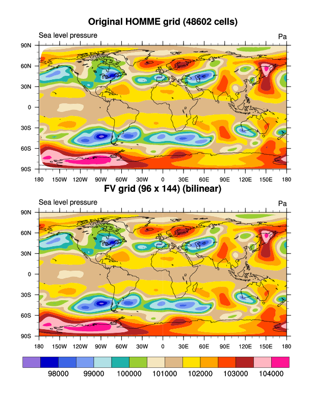
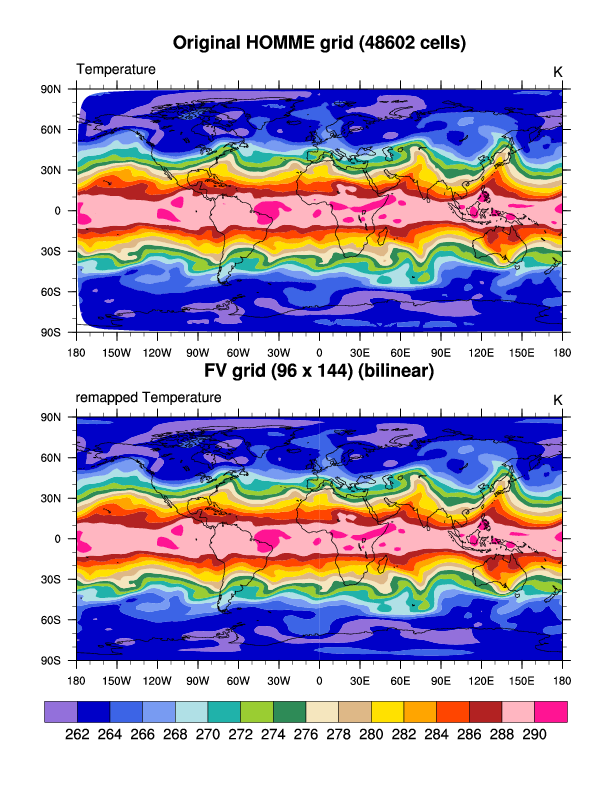 ESMF_regrid_18.ncl:
This example shows how to regrid two variables (PSL and T) on a HOMME cubed-sphere (unstructured) finite volume grid (48602 cells) to a 96 x 144 finite volume (FV) rectilinear grid.
Once the first variable has been regridded using ESMF_regrid, you will have a NetCDF weights file. You can then use this weights file to regrid the second variable using ESMF_regrid_with_weights. This can be much faster than using ESMF_regrid again.
 ESMF_regrid_19.ncl:
This example shows how to regrid data on a HOMME cubed-sphere (unstructured) grid to POP curvilinear gx1v3 grid (384 x 320).
In this case, the POP grid was retrieved from an old weights file from a previous regridding that went from a 1x1 degree grid to a POP grid.
The destination lat/lon arrays on this weights file have corresponding names "yc_b" and "xc_b", and are one-dimensional. You have to reshape these 1D arrays to their original 2D structure using the "dst_grid_dims" variable on the file. The POP weights file also contains a mask grid called "mask_b" that you must apply via the special "DstMask2D" option.
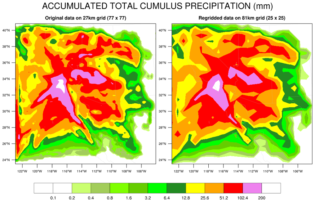 ESMF_regrid_20.ncl:
This example shows how to regrid from a 27km WRF grid to a coarser 81km WRF grid using bilinear interpolation.
The color scheme used here is similar to the one used on the precipitation page of the WRF-ARW Online Tutorial. Set USE_WRF_COLORS to False if you want to "WhViBlGrYeOrRe" color table and a slightly different set of contour levels.
 ESMF_regrid_21.ncl:
This example shows how to regrid from random (unstructured) data to a 0.1 degree grid.
Since this grid is not global, it is important to set the special "DstLLCorner" and "DstURCorner" resources to further zoom in on the 0.1 degree grid that the original data lies on. If you don't set these resources, then a global 0.1 degree grid will be created, causing the regridding to take a MUCH longer time.
 ESMF_regrid_22.ncl:
This example shows how to regrid from data on a curvilinear grid that contains missing lat/lon values, to data on a curvilinear grid that covers a much smaller region.
Since the source grid contains missing values, it's important to set the SrcMask2D option:
  Opt@SrcMask2D         = where(ismissing(src_lat2d).or.\
                                ismissing(src_lon2d),0,1)
For plotting the data on the original grid, it is important to set:
res@trGridType = "TriangularMesh"
so it handles these missing values correctly.
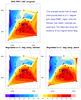
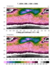
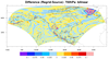
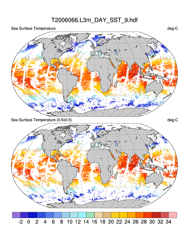 ESMF_regrid_23.ncl: This
example was taken from the HDF examples
page. It shows how to regrid data from a 9 km MODIS Aqua Level-3
HDF4 file to a 0.5 degree grid. The file attributes contain the
geographical information, which is used to generate coordinate
variables for the source grid.
ESMF_regrid_23.ncl: This
example was taken from the HDF examples
page. It shows how to regrid data from a 9 km MODIS Aqua Level-3
HDF4 file to a 0.5 degree grid. The file attributes contain the
geographical information, which is used to generate coordinate
variables for the source grid.
The generation of the required files for regridding can be slow for this data, so once you have the "MODIST_to_0.5deg.nc" weights file, you can use ESMF_regrid_with_weights instead of ESMF_regrid to do the regridding. Look for HAVE_WGTS in the script for more information.

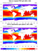
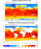
 ESMF_regrid_24.ncl: This
example shows how to regrid data from a POP curvilinear gx1v3 grid
(384 x 320) to a 1.0 degree world grid. It plots sea water potential
temperature on the new grid.
ESMF_regrid_24.ncl: This
example shows how to regrid data from a POP curvilinear gx1v3 grid
(384 x 320) to a 1.0 degree world grid. It plots sea water potential
temperature on the new grid.
Note: Conservative interpolation will fail because grid vertex information needed by the ESMF software is not available.
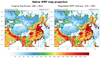
 ESMF_regrid_25.ncl /
ESMF_wgts_25.ncl: This
example shows how to regrid CLM data on the 'ne30' to a finite volume grid.
ESMF_regrid_25.ncl /
ESMF_wgts_25.ncl: This
example shows how to regrid CLM data on the 'ne30' to a finite volume grid.
Note 1: For some reason, in the CLM, grid
Note 2: Conservative interpolation will fail because grid vertex information
needed by the ESMF software is not available.
Note 3: Once you have the weights file generated by
ESMF_regrid_25.ncl, you can
use ESMF_regrid_with_weights to do
the regridding using this file.
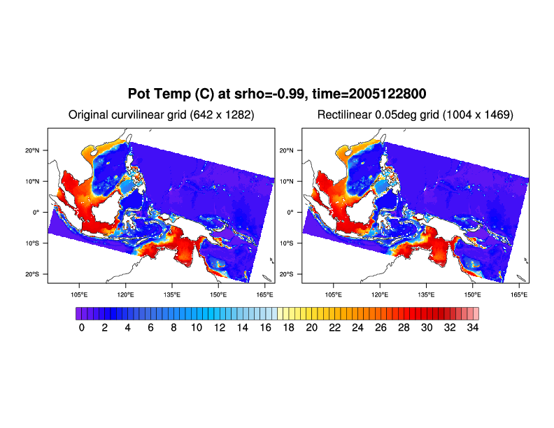 ESMF_regrid_26.ncl:
This shows how to regrid a ROMS model output to a rectilinear grid.
The ROMS grid information and the model variable output are
contained on separate files.
This specific version of ROMS is for the "Coral configuration."
The original grid has 5km spacing. The rectilinear grid is set to 0.05
degree spacing which corresponds to approximately 5km (~0.05*111km).
ESMF_regrid_26.ncl:
This shows how to regrid a ROMS model output to a rectilinear grid.
The ROMS grid information and the model variable output are
contained on separate files.
This specific version of ROMS is for the "Coral configuration."
The original grid has 5km spacing. The rectilinear grid is set to 0.05
degree spacing which corresponds to approximately 5km (~0.05*111km).
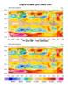
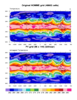
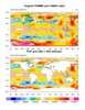
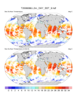
 ESMF_regrid_27.ncl:
This example shows how to regrid variables from a suite of ECMWF files
that contain an Operational Model Analysis grid with a 1280 x 2560
regular Gaussian grid to a lower resolution 2.5 degree grid.
ESMF_regrid_27.ncl:
This example shows how to regrid variables from a suite of ECMWF files
that contain an Operational Model Analysis grid with a 1280 x 2560
regular Gaussian grid to a lower resolution 2.5 degree grid.
The results are written to individual NetCDF files using the efficient method.
Only one weight file needs to be generated here, so ESMF_regrid is used to create the weights file, and then ESMF_regrid_with_weights is used to do the regridding of all the variables. If you were to run the script again with a different set of files that have the same grids, you can set "GEN_WEIGHTS" to False so the weights file is not regenerated.
Just for something different, the "cb_rainbow_inv" color map was used here. This color map may be useful for color blindness and color deficient viewers.
 ESMF_regrid_28.ncl:
The demonstrates how to regrid variables on a rectilinear grid onto
a POP curvilinear grid. The source variable is type short and
must be unpacked prior to regridding. Further, only the 1st time
step is read because only the spatial information (latitudes
and longitudes) is needed for weight generation. POP variables have no values
over land. Hence, a variable from the target POP file is read
and used to generate a mask.
ESMF_regrid_28.ncl:
The demonstrates how to regrid variables on a rectilinear grid onto
a POP curvilinear grid. The source variable is type short and
must be unpacked prior to regridding. Further, only the 1st time
step is read because only the spatial information (latitudes
and longitudes) is needed for weight generation. POP variables have no values
over land. Hence, a variable from the target POP file is read
and used to generate a mask.
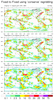
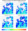
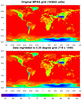
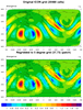
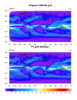
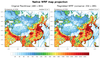
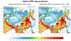
 ESMF_regrid_29.ncl /
ESMF_wgts_29.ncl:
These scripts show how you can use a two-step process to regrid WRF data.
ESMF_regrid_29.ncl /
ESMF_wgts_29.ncl:
These scripts show how you can use a two-step process to regrid WRF data.The ESMF_regrid_29.ncl script creates two weights files: (1) WRF grid to a rectilinear grid and (2) rectilinear grid back to the original WRF grid. A 3-panel plot is created: (1) an arbitrary variable plotted on the original WRF grid, (2) the same variable regridded to the rectilinear grid, (3) the same variable regridded from the rectilinear grid back to the WRF grid.
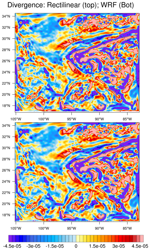
The ESMF_wgts_29.ncl script shows how you can now use the WRF-to-rectilinear weights file created by the previous script to interpolate the zonal and meridional wind components to a rectilinear grid. It then uses the uv2dv_cfd function to compute divergence on a rectilinear grid and then regrids this quantity back onto the original WRF grid using the rectilinear-to-WRF weight file generated by the previous script.
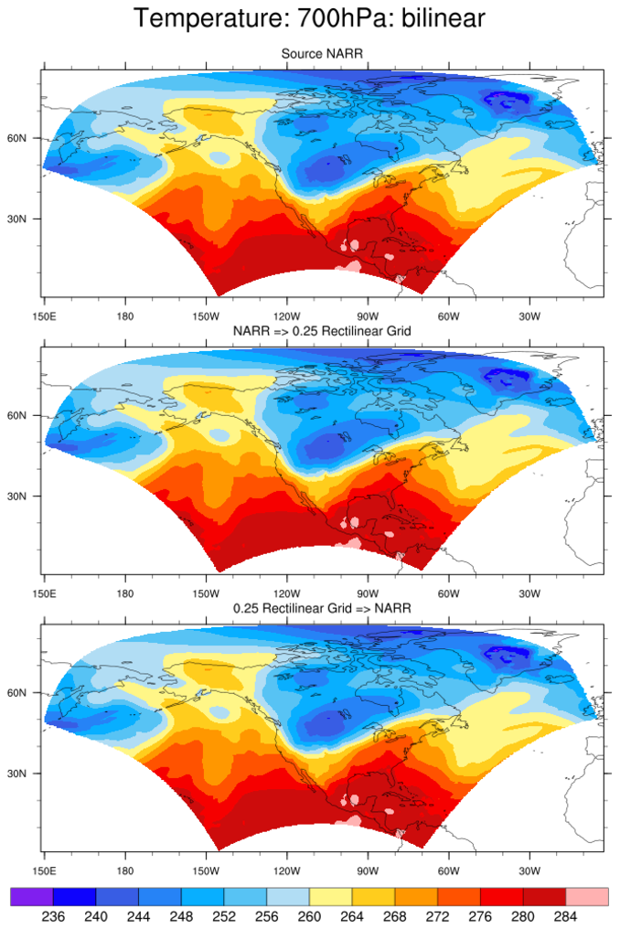
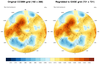
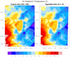
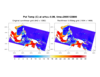
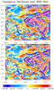
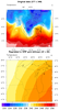
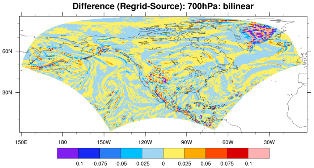 ESMF_wgts_30.ncl:
This script regrids a NARR grid which is a curvilinear grid to a 0.25 rectilinear grid (Part A).
Then for illustration it regrids the rectilinear grid back to the original NARR grid (Part B).
The rectilinear->NARR section (Part B) could easily be extracted and used as a template to regrid any
rectilinear grid to the NARR grid.
ESMF_wgts_30.ncl:
This script regrids a NARR grid which is a curvilinear grid to a 0.25 rectilinear grid (Part A).
Then for illustration it regrids the rectilinear grid back to the original NARR grid (Part B).
The rectilinear->NARR section (Part B) could easily be extracted and used as a template to regrid any
rectilinear grid to the NARR grid.
The rightmost plot shows the difference after reinterpolating the 0.25 rectilinear gridded field back to the original curvilinear grid. The differences are quite small and are expected: (a) the 0.25 grid is slightly coarser than the original NARR grid; (b) the largest magnitudes are over regions affected by topography. If (say) 200 hPA had been chosen, the differences would be even smaller.
Use ESMF_wgts_30.ncl to generate two weight files: (a) NARR grid to rectilinear grid; (b) rectilinear to NARR grid. This is done only once for each grid.
NARR Example 5 shows how a user could use an ESMF-generated weight file to quickly interpolate the NARR to a rectilinear grid and then create cross-sections.
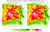
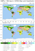
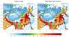
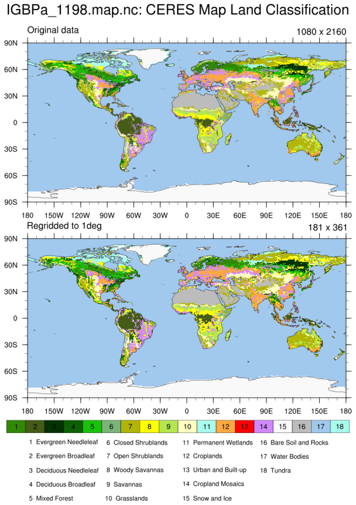 ESMF_regrid_31.ncl:
This script regrids IGBP vegetation categorical data which is on
a high-resolution 1080 x 2160 grid, to a 1 degree lat/lon grid.
ESMF_regrid_31.ncl:
This script regrids IGBP vegetation categorical data which is on
a high-resolution 1080 x 2160 grid, to a 1 degree lat/lon grid.
Because of the size of the grid, this example takes about 14 minutes to run on a Mac system. Once you have the weights file however, you can regrid data on the same grid using the weights file. See the "have_wgts_file" variable in the script.
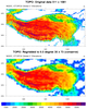
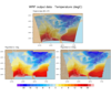
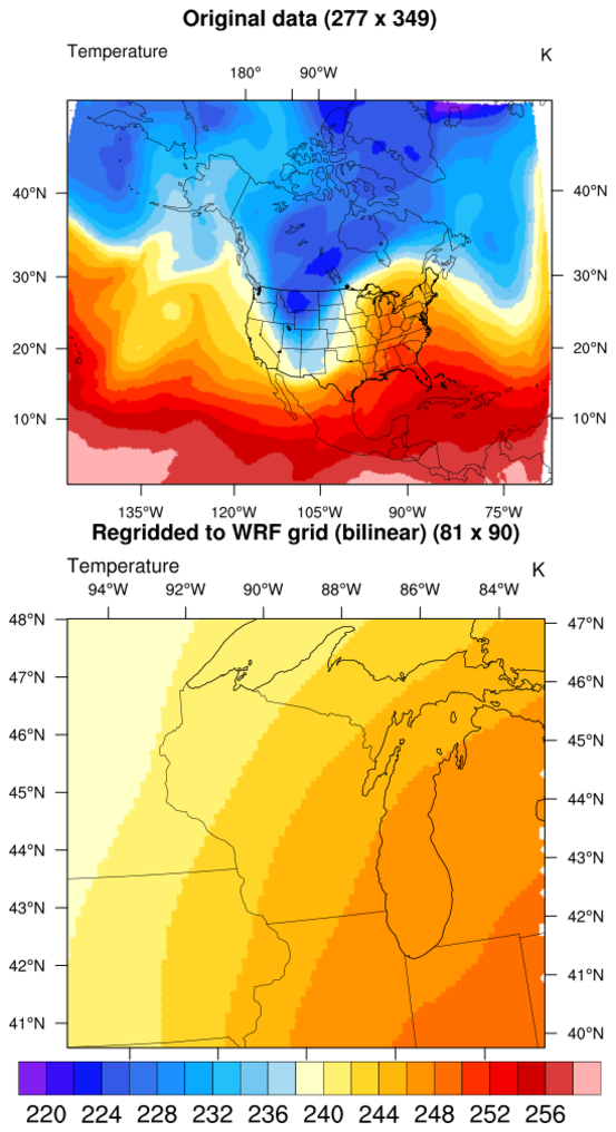
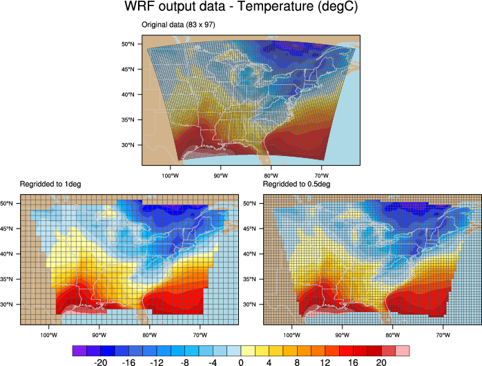 ESMF_regrid_32.ncl: This
example regrids WRF output temperature data to both a 1.0 and 0.5 degree
grid, and compares them in a panel plot.
ESMF_regrid_32.ncl: This
example regrids WRF output temperature data to both a 1.0 and 0.5 degree
grid, and compares them in a panel plot.
The gsn_coordinates procedure is used to draw the lat/lon grid on all three plots.
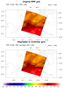
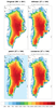
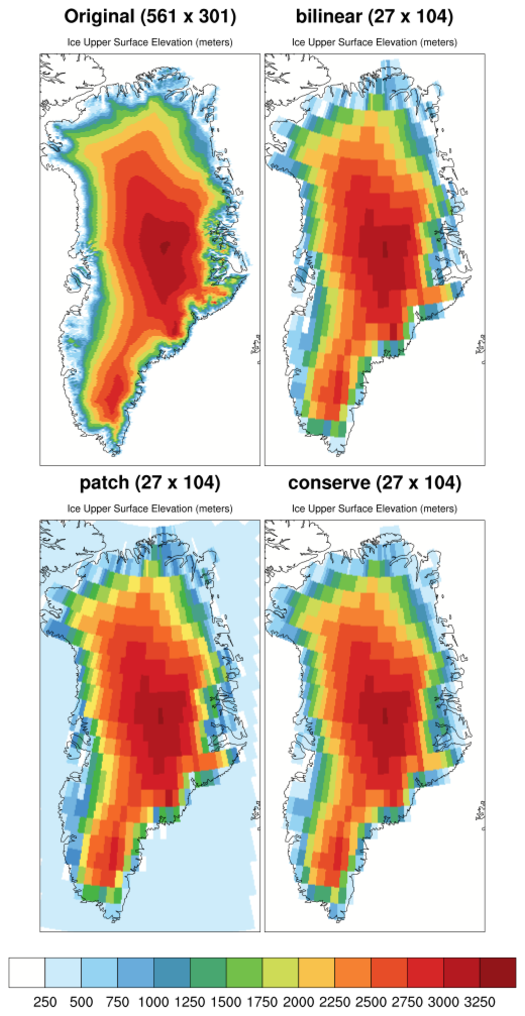 ESMF_regrid_33.ncl: This
example regrids the 'gland5.nc' (Greenland Developmental Data Set: Greenland_5km_dev1.1.nc)
data on a very high resolution 5km grid to a 0.5 degree grid using the bilinear, patch and conserve
interpolation methods. A subsequent run generated a separate regrid weight file for a 1x1 resolution.
See: gland_2/3
for application of these weight files.
ESMF_regrid_33.ncl: This
example regrids the 'gland5.nc' (Greenland Developmental Data Set: Greenland_5km_dev1.1.nc)
data on a very high resolution 5km grid to a 0.5 degree grid using the bilinear, patch and conserve
interpolation methods. A subsequent run generated a separate regrid weight file for a 1x1 resolution.
See: gland_2/3
for application of these weight files.
 ESMF_regrid_34.ncl:
This interpolates data on a NARR grid to a WRF grid. Here, the WRF grid covers a much smaller area than the source NARR grid. This is a curvilinear to curvilinear interpolation.
ESMF_regrid_34.ncl:
This interpolates data on a NARR grid to a WRF grid. Here, the WRF grid covers a much smaller area than the source NARR grid. This is a curvilinear to curvilinear interpolation.
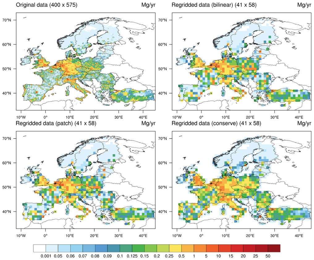 ESMF_regrid_35.ncl:
Using the ESMF 'bilinear', 'patch' and 'conserve' methods to interpolate a high-resolution
(0.1x0.1) rectilinear regional grid a lower resolution (1x1) rectilinear grid.
This is similar to several
other ESMF examples. However, the source data is a 'bit fractal' in nature. It illustrates
the results of the three methods.
ESMF_regrid_35.ncl:
Using the ESMF 'bilinear', 'patch' and 'conserve' methods to interpolate a high-resolution
(0.1x0.1) rectilinear regional grid a lower resolution (1x1) rectilinear grid.
This is similar to several
other ESMF examples. However, the source data is a 'bit fractal' in nature. It illustrates
the results of the three methods.
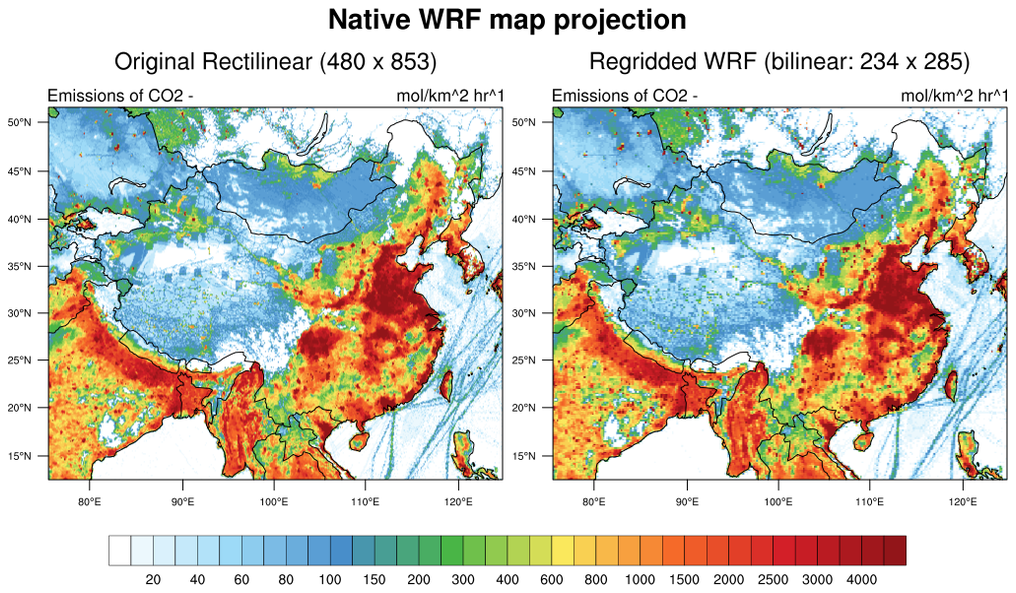
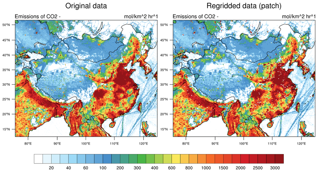
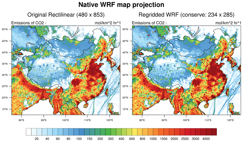
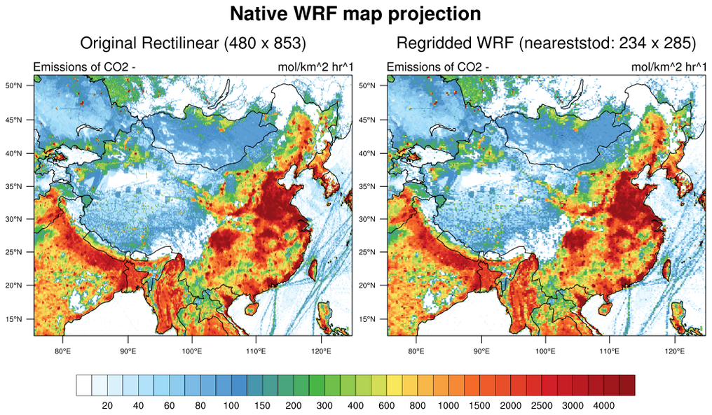 ESMF_regrid_36.ncl:
Interpolate data from a high resolution (0.1x0.1 [1800x3600]) global grid
to a regional curvilinear (WRF) grid using 'bilinear', 'patch', 'nearestod',
and 'conserve' methods. NCL's
coordinate
subscripting is used to extract an area subset surrounding China. This reduces the
interpolation time.
ESMF_regrid_36.ncl:
Interpolate data from a high resolution (0.1x0.1 [1800x3600]) global grid
to a regional curvilinear (WRF) grid using 'bilinear', 'patch', 'nearestod',
and 'conserve' methods. NCL's
coordinate
subscripting is used to extract an area subset surrounding China. This reduces the
interpolation time.
The wrf_map_resources function is used to extract the WRF map projection information defined on the WRF file.
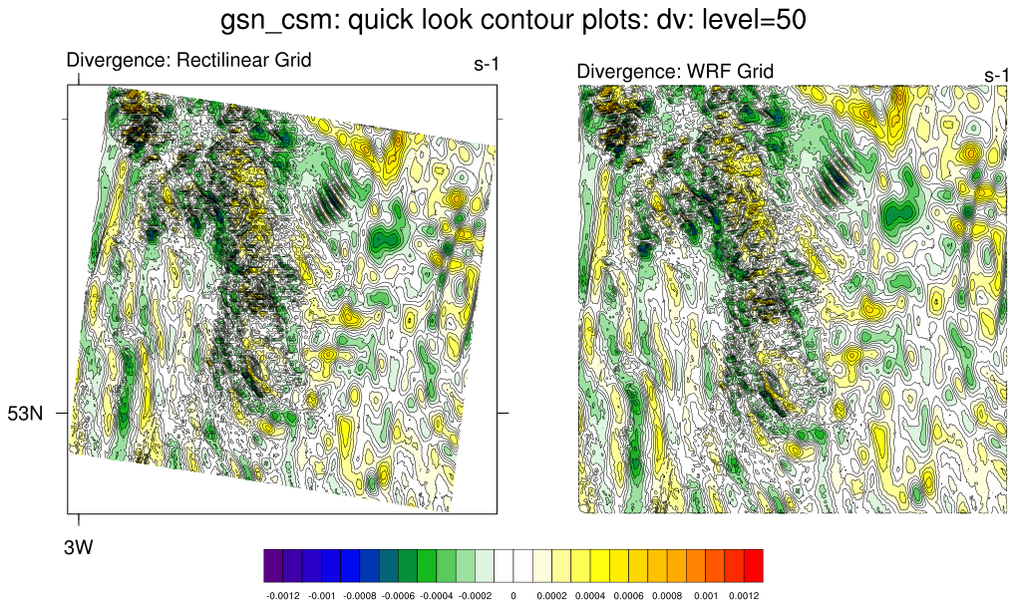
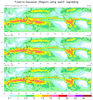
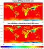
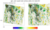
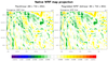
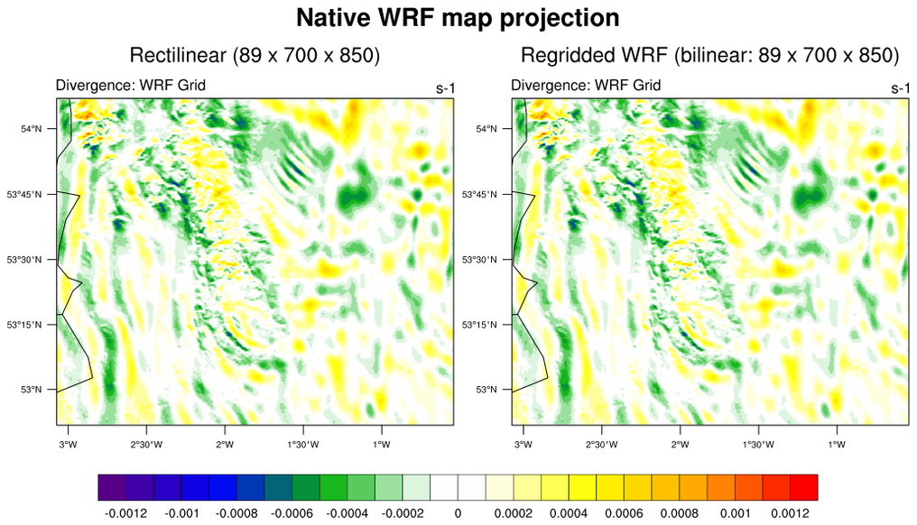 ESMF_regrid_37.ncl:
The is similar to the ESMF_wgts_29.ncl script. It regrids the WRF's zonal
and meridional wind components onto a rectilinear grid. It then uses
the uv2dv_cfd function to compute divergence on the rectilinear
grid and then regrids the divergence back onto the original WRF grid.
ESMF_regrid_37.ncl:
The is similar to the ESMF_wgts_29.ncl script. It regrids the WRF's zonal
and meridional wind components onto a rectilinear grid. It then uses
the uv2dv_cfd function to compute divergence on the rectilinear
grid and then regrids the divergence back onto the original WRF grid.