NCL Home>
Application examples>
Models ||
Data files for some examples


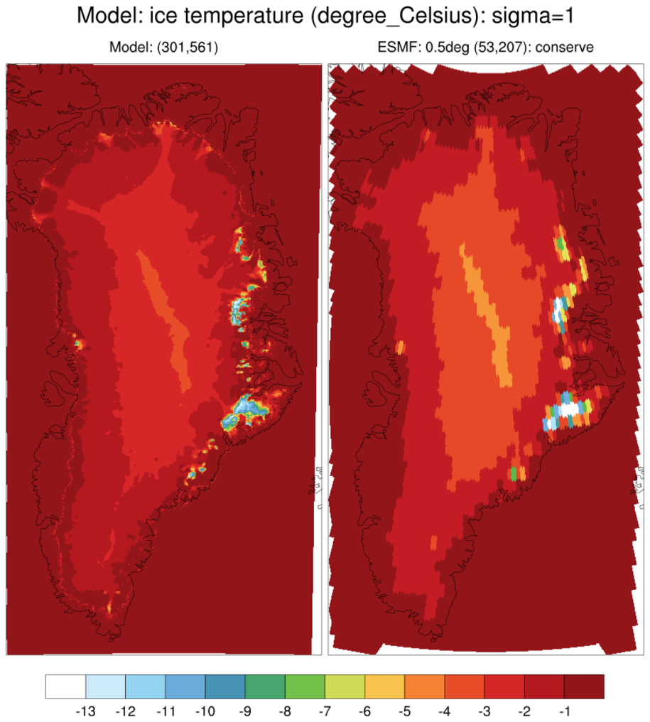
 gland_cism_1.ncl:
Read a CISM Greenland ice model output file and regrid to 0.5 degrees using the
ESMF example 33
conserve 0.5 weight file.
gland_cism_1.ncl:
Read a CISM Greenland ice model output file and regrid to 0.5 degrees using the
ESMF example 33
conserve 0.5 weight file.
Example pages containing: tips | resources | functions/procedures
NCL Graphics: CESM Ice Model, CISM (Community Ice Sheet Model)
The Community Ice Sheet Model (CISM)
is a next-generation ice sheet model used for predicting ice sheet evolution and sea level
rise in a changing climate. It serves as the ice dynamics component of the Community Earth
System Model (CESM), which is one of the first global climate models to include coupled,
dynamic ice sheets.
Many of these plots use the gsn_csm_contour_map_polar
high-level plot interface. More examples of its use are available on the
polar example page.
1D coordinate variables
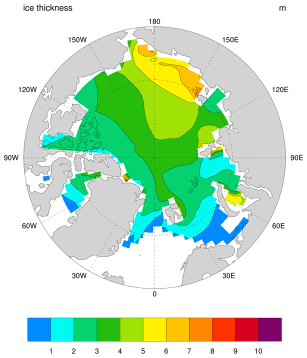
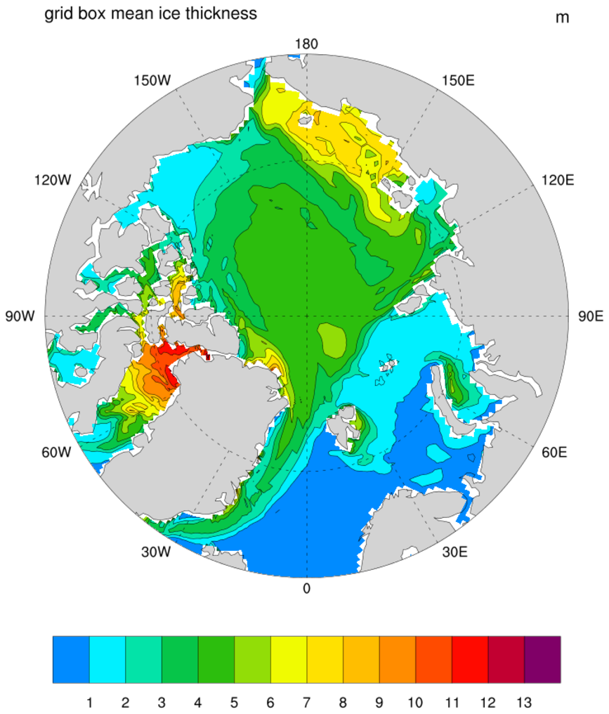
ice_1.ncl: A simple plot showing ice thickness with a spectrum of color.gsn_csm_contour_map_polar is the plot interface that draws contours on a polar stereographicmap.
cnFillOn = True, Turns on the color fill.
1D coordinate variables
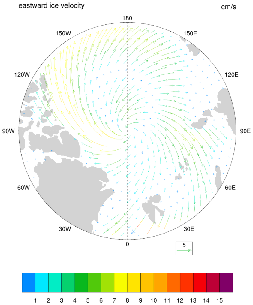
ice_2.ncl: A polar vector plot of ice velocity.gsn_csm_vector_map_polar is the plot interface that draws vectors on a polar stereographic map.
vcMonoLineArrowColor = False, Turns on color vectors.
To turn on curly vectors, set the resource vcGlyphStyle = "CurlyVector"
2D coordinate variables
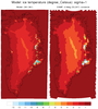
ice_3.ncl: Demonstrates plotting ice variables from file that contain 2D coordinate variables. There are many more example of this technique on the pop ocean page.As of NCL version 4.2.0.a025, data that has 2D lat/lon coordinates can be plotted directly in physical space. To do this, simply read in the coordinates and assign them the following attributes:
       lat2d     = f->TLAT
       lon2d     = f->TLONG
       t@lon2d   = lon2d
       t@lat2d   = lat2d


CICE Tripole Grid
ice_4.ncl: This 3 frame plot demonstrates a solution to the gap that appears along a line between the two northern poles for data represented on the CICE T-fold Tripole grid. Thanks to Petteri Uotila of CSIRO Marine & Atmospheric Research in Aspendale, Victoria, Australia for providing this solution. The first frame demonstrates the problem when the data is plotted normally using the T-fold grid coordinates. The second frame draws the same data but switches to the U-fold grid coordinates that are also present in the file. This rendering eliminates the gap but slightly misplaces the data in the coordinate space. The third frame shows the solution obtained by adding the top row of the U-fold grid to the T-fold grid and simply repeating the top row data in a row added to the data array.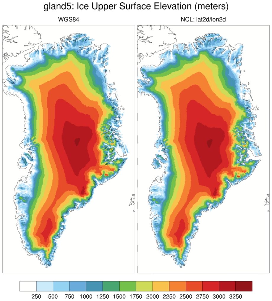

gland
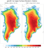
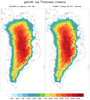
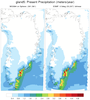
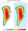
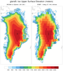
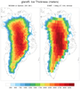
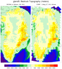
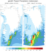
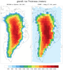
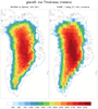
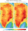
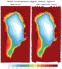
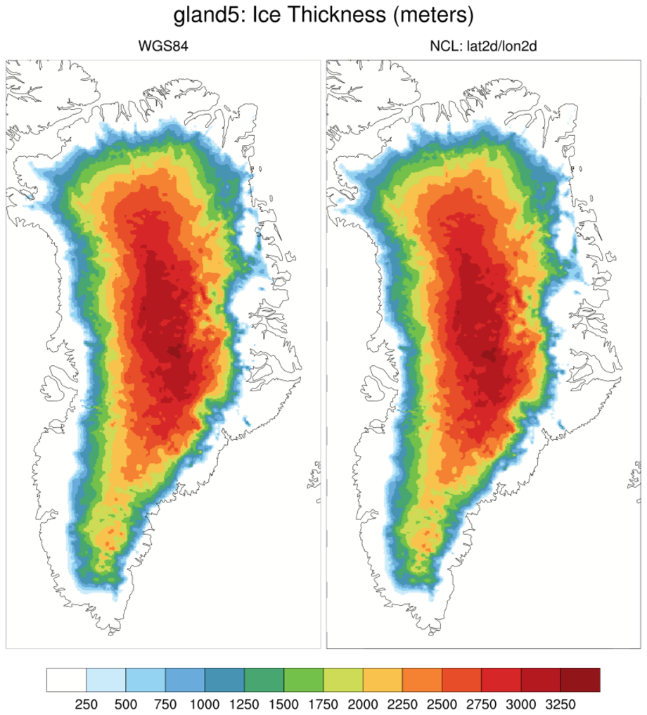
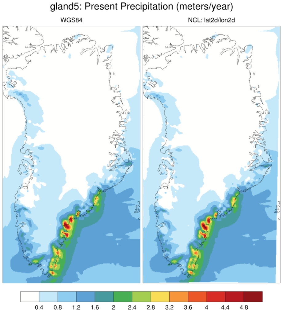
gland_1.ncl: The data on this file are extracted from Greenland Developmental Data Set: Greenland_5km_dev1.1.nc. The source is on a geodetic datum coordinate system. These are defined on an ellipsoid. NCL graphiccal mappings assume a sphere. As a result, there can be slight differences between the the WGS84 rendering and that created by NCL. The four plots show the 'native' plot on the left and the NCL's spherically based mapping of the variable. This differences are most clearly observed via the 'topg' variable.
        char mapping ;
                mapping:ellipsoid = "WGS84" ;
                mapping:false_easting = 0. ;
                mapping:false_northing = 0. ;
                mapping:grid_mapping_name = "polar_stereographic" ;
                mapping:latitude_of_projection_origin = 90. ;
                mapping:standard_parallel = 71. ;
                mapping:straight_vertical_longitude_from_pole = -39. ;
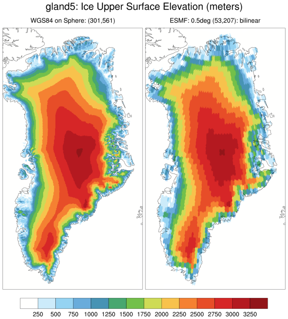

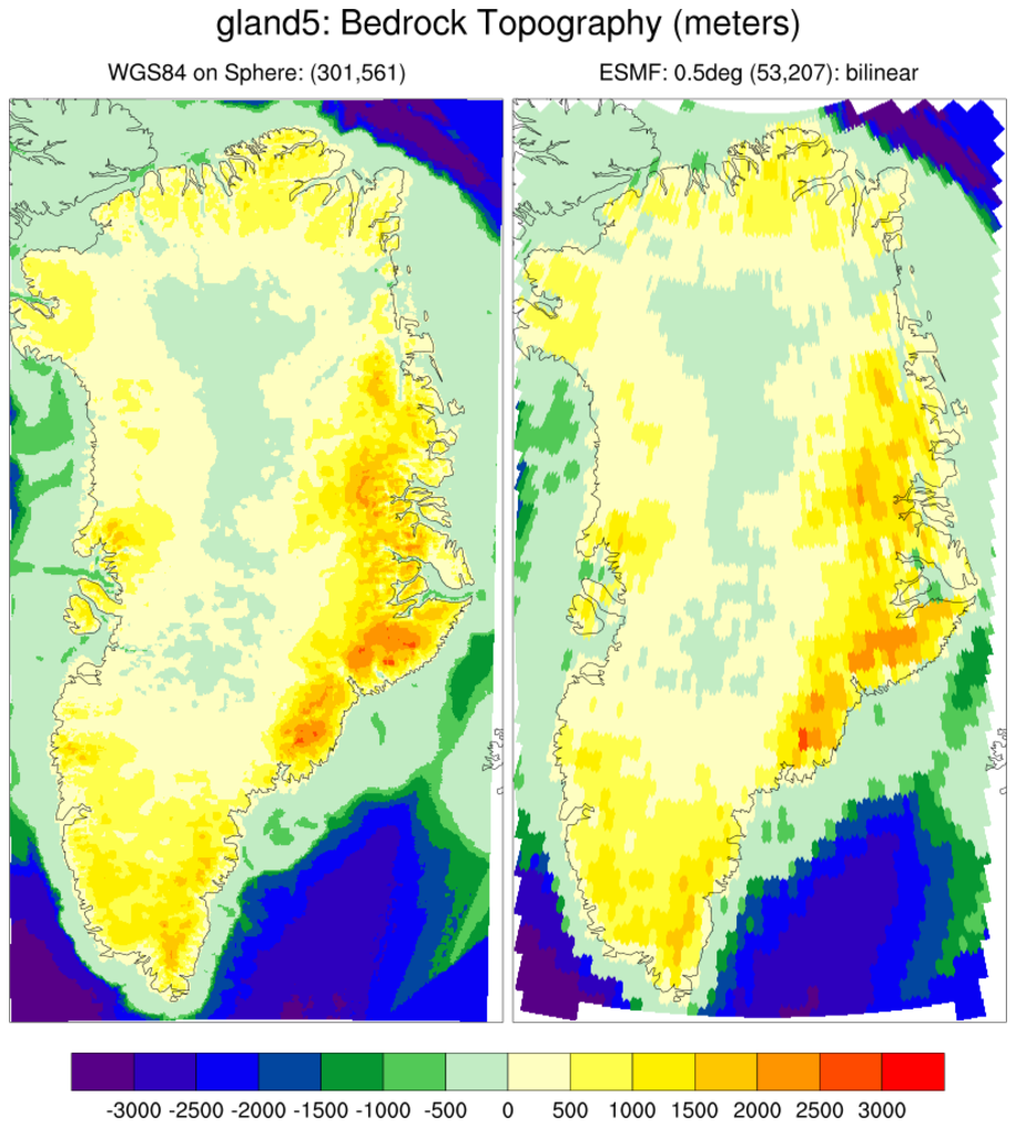
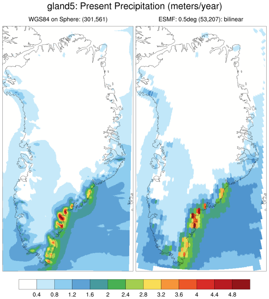
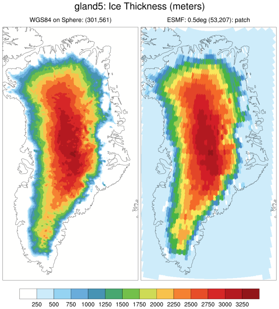

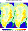
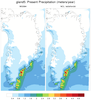
gland: ESMF 0.5
gland_2.ncl: This uses the 0.5x0.5 weight files generated in ESMF example 33. The raw data are read and regridded for each variable. The first four show the four variables interpolated via bilinear interpolation. For comparison, the rightmost two plots show the "Ice Thickness" variable interpolated using the patch and conserve methods.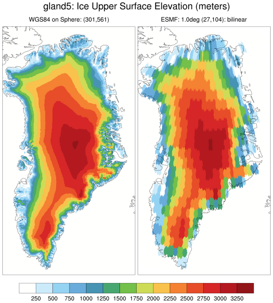
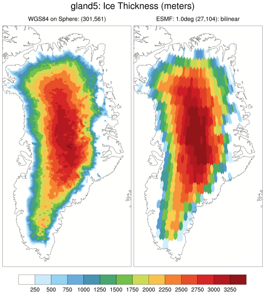
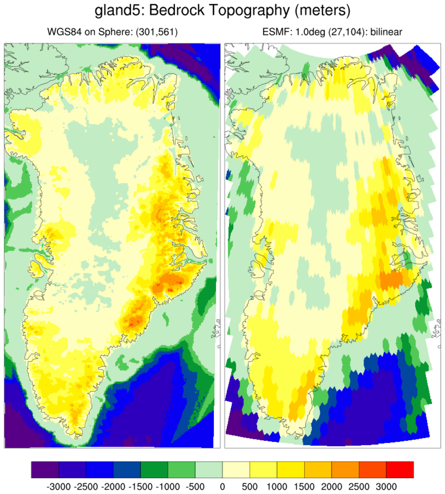
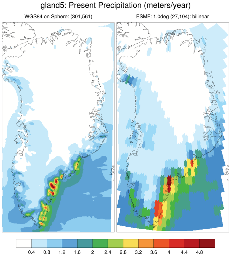

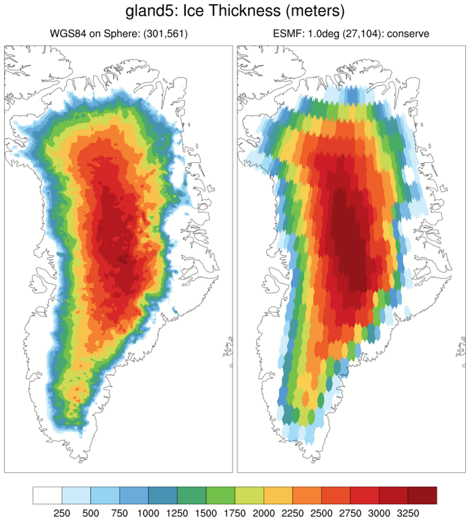
gland: ESMF 1.0
gland_3.ncl: Same as the previous example except using the 1.0deg (1x1) weight files.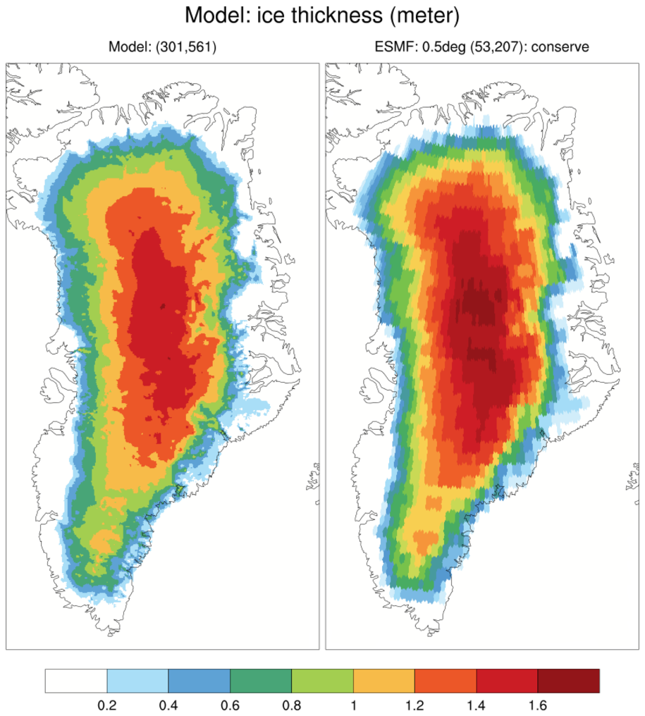


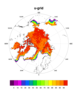
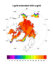
 gland_cism_1.ncl:
Read a CISM Greenland ice model output file and regrid to 0.5 degrees using the
ESMF example 33
conserve 0.5 weight file.
gland_cism_1.ncl:
Read a CISM Greenland ice model output file and regrid to 0.5 degrees using the
ESMF example 33
conserve 0.5 weight file.