NCL Graphics: POP Ocean Model

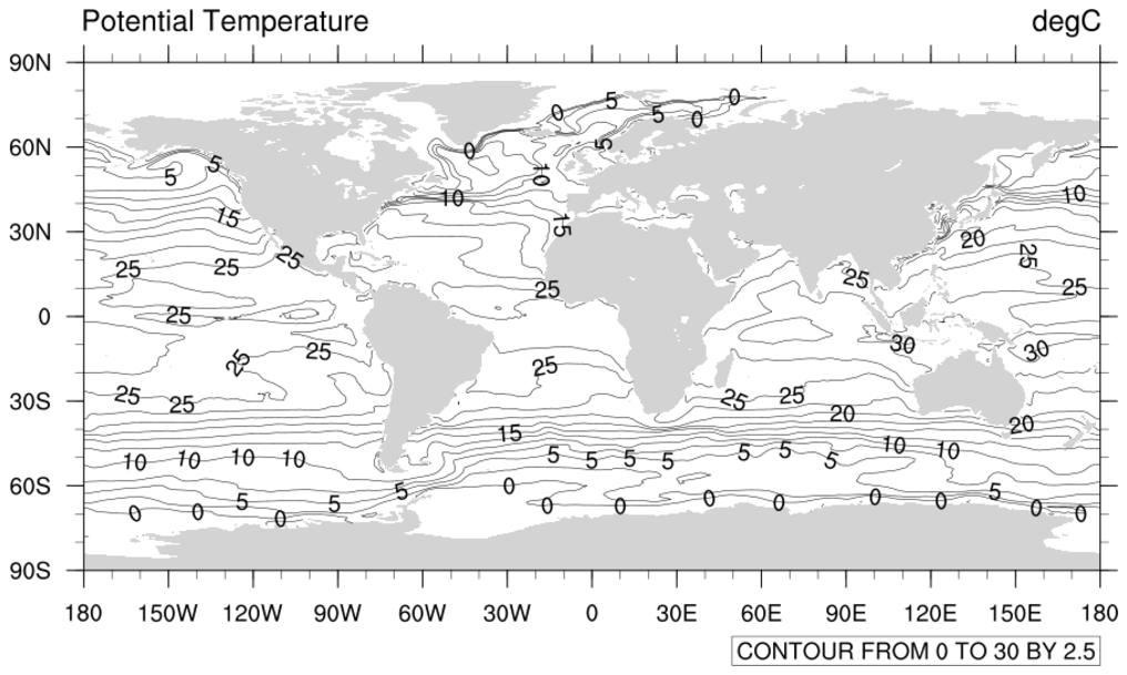
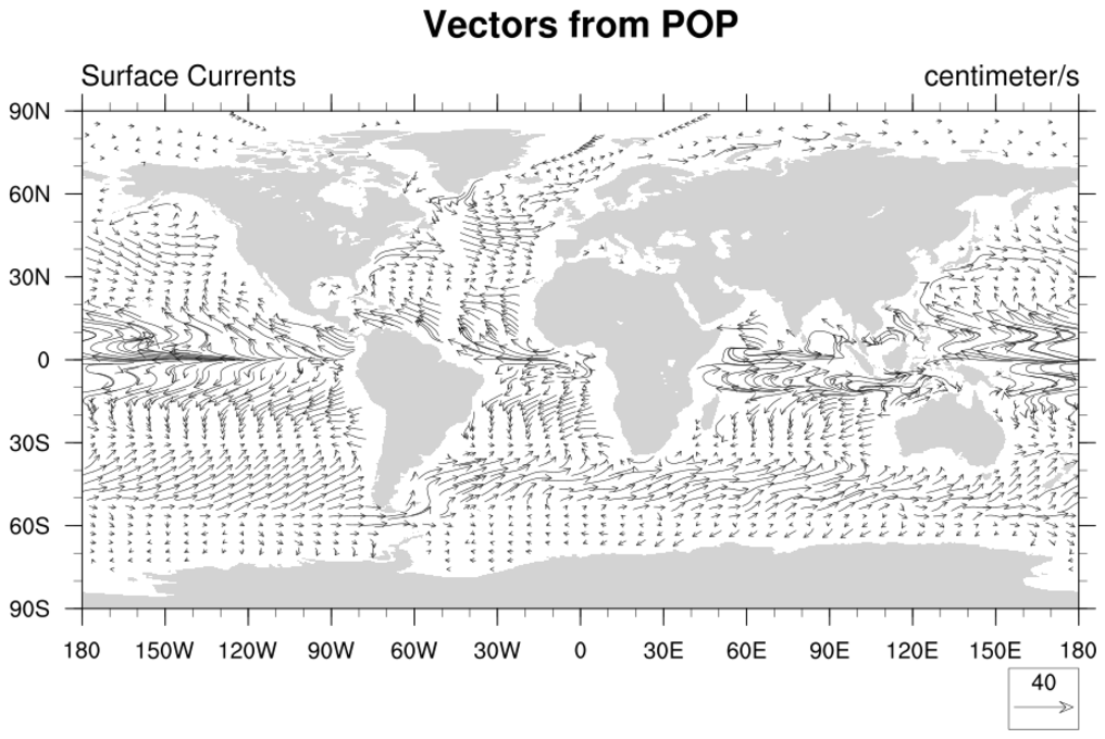
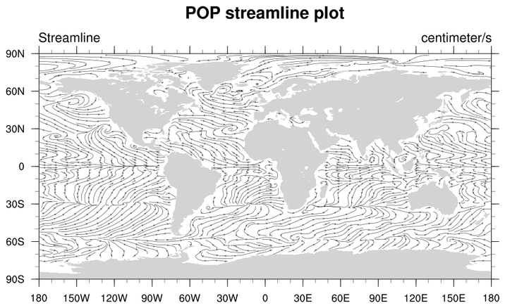
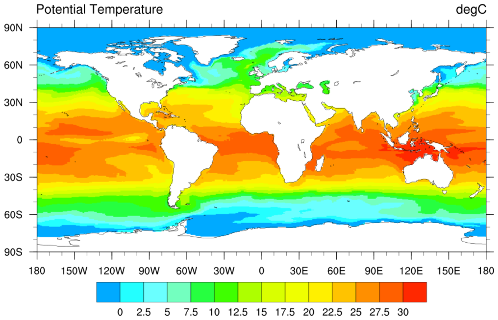
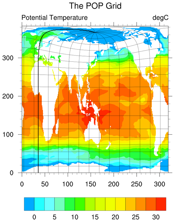
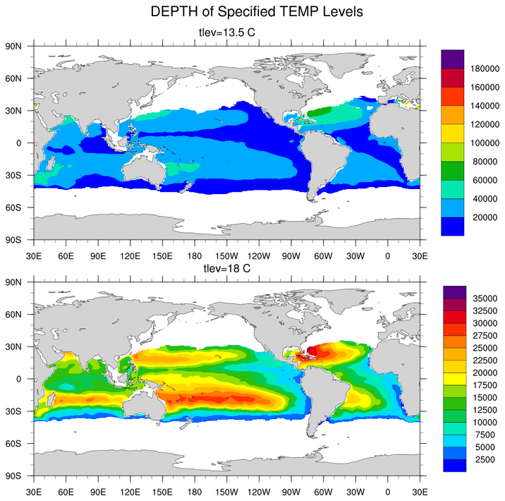
POP variables (scalar and vector) can be plotted directly. Numerous examples are shown below.

In some cases, the user may wish to interpolate to a different grid. The Grid Conversions section below illustrates how the interpolation can be done within the NCL environment. Generally, the remapping to different grids requires weight files.

Several POP specific functions are available:

1. moc_globe_atl: Estimate the POP model Meridional Overturning Circulation (MOC).

2. rho_mwjf: Given a specified range for potential temperature and salinity the ocean water density can be calculated via rho_mwjf. Sample usage and generated plots may be seen here.

CAUTION: The yyyy-mm within the POP file name and the time variable contained within the file may not necessarily agree with one another. This can be confusing and lead to erroneous temporal assignment(s). Consider a file named "sample.pop.h.0280-01.nc". The file 'yyyy-mm' is 280-01 (January, 280).

 f = addfile("g.b29.01.pop.h.0280-01.nc","r")
 time = f->time
 print(time)

     Variable: time
     Type: double
              [snip] 
     Dimensions and sizes:	[time | 1]
     Coordinates: 
              time: [102231..102231]
     Number Of Attributes: 4
       long_name :	time
     units :	days since 0000-01-01 00:00:00
     bounds :	time_bound
     calendar :	noleap
     
     (0)     102231

 date = cd_calendar(time, 0)                  
 print(date)
     
     Variable: date
     Dimensions and sizes:   [1] x [6]
     Coordinates: 
     Number Of Attributes: 1
    calendar :    noleap
  (0,0)   280         
  (0,1)    2 
              [snip] 

The variable 'time' indicates 280-02 or February, 280 which is not consistent with the file name of 280-01 or January, 280. How to deal with this? One approach is to use the 'time_bound' variable.

 time_bound = f->time_bound  
 print(time_bound)

     Variable: time_bound
     Type: double
     Total Size: 16 bytes
                 2 values
     Number of Dimensions: 2
     Dimensions and sizes:   [time | 1] x [d2 | 2]
     Coordinates: 
                 time: [102231..102231]
     Number Of Attributes: 2
       long_name :   boundaries for time-averaging interval
       units :       days since 0000-01-01 00:00:00
  (0,0)   102200     <==== this is the beginning of the averaging time
  (0,1)   102231     <==== this is the same as 'time'

 time = (/ time_bound(:,0) /)          ; override values with lower bound  
 print(time)                           ; <=== 102200
 date = cd_calendar(time, 0) 
 print(date)                           

     Variable: date
     Type: float
     Total Size: 24 bytes
                 6 values
     Number of Dimensions: 2
     Dimensions and sizes:   [1] x [6]
     Coordinates: 
     Number Of Attributes: 1
       calendar :    noleap
  (0,0)   280
  (0,1)    1 

------------------------------------------------------------------------------>
------------------------------------------------------------------------------>
Another (better) approach is to average the time_bnd variable to get the
'center-of-mass' of the observations. 

 time       = f->time
 time_bound = f->time_bound  
 time       = (/ (time_bound(:,0)+time_bound(:,1))*0.5 /)    ; override values with average

For NCL application, one could reassign the 'time' coordinate variable
associated with a variable:

 temp       = f->TEMP
 temp&time  = (/ time  /)     ; reasign with more appropriate values