       lat2d     = f->TLAT
       lon2d     = f->TLONG
       t@lon2d   = lon2d
       t@lat2d   = lat2d
To learn more about vectors, please view the
vector example page.
NCL Home>
Application examples>
Models ||
Data files for some examples
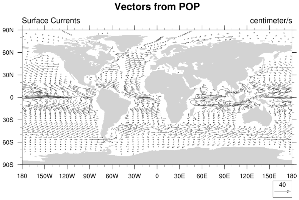
 popvec_1.ncl: A basic vector plot.
UVEL and VVEL are NOT zonal and meridional velocities in the lat/lon sense. They are velocities with respect to the model grid, which is locally rotated by ANGLE radians with respect to lat/lon directions. So to convert to zonal & meridional velocities, you need to project UVEL and VVEL onto zonal & meridional directions. Here's how :
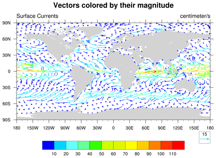
 popvec_2.ncl: Color vectors and use a
simpler thinning scheme.
popvec_2.ncl: Color vectors and use a
simpler thinning scheme.
vcMonoLineArrowColor = False, Turns on the color vectors
vcMinDistanceF will thin the vectors just like the subsampling in example 1. This is a easier method.
 popvec_3.ncl: A zoom plot
vcRefAnnoOrthogonalPosF = -1.0, Moves the reference vector up into the plot.
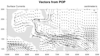
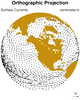 popvec_4.ncl: A different
projection.
You are not limited to cylindrical equidistant projections. There are
several projections to choose from.
popvec_4.ncl: A different
projection.
You are not limited to cylindrical equidistant projections. There are
several projections to choose from.
This is an orthographic projection.
Example pages containing:
tips |
resources |
functions/procedures
NCL Graphics: POP Vectors
POP data that have 2D lat/lon coordinates
can be plotted directly in physical space. To do this, simply read in
the coordinates and assign them the following attributes:
 popvec_1.ncl: A basic vector plot.
UVEL and VVEL are NOT zonal and meridional velocities in the lat/lon sense. They are velocities with respect to the model grid, which is locally rotated by ANGLE radians with respect to lat/lon directions. So to convert to zonal & meridional velocities, you need to project UVEL and VVEL onto zonal & meridional directions. Here's how :
    true_zonal_velocity = cos(ANGLE) * UVEL - sin(ANGLE) * VVEL
    true_merid_velocity = sin(ANGLE) * UVEL + cos(ANGLE) * VVEL
If you wish to convert regular lat/lon data to the pop grid, the
following is used:
      uPop =  u*cos(rot) + v*sin(rot)
      vPop = -u*sin(rot) + v*cos(rot)
popvec_2.ncl: Color vectors and use a
simpler thinning scheme.
vcMonoLineArrowColor = False, Turns on the color vectors
vcMinDistanceF will thin the vectors just like the subsampling in example 1. This is a easier method.
 popvec_3.ncl: A zoom plot
vcRefAnnoOrthogonalPosF = -1.0, Moves the reference vector up into the plot.
 popvec_4.ncl: A different
projection.
You are not limited to cylindrical equidistant projections. There are
several projections to choose from.
popvec_4.ncl: A different
projection.
You are not limited to cylindrical equidistant projections. There are
several projections to choose from.
This is an orthographic projection.