NCL Home>
Application examples>
Data Analysis ||
Data files for some examples
Example pages containing:
tips |
resources |
functions/procedures
NCL: Regridding
Regridding is the process of interpolating from a source grid (SRC), to a
destination grid (DST). For
rectilinear,
grids this may be represented as
                 SRC(ys,xs) ==> DST(yd,xd)
where
                 ys,xs rectilinear
There are numerous
regridding functions
available in NCL. In NCL version
6.1.0,
new regridding capabilities available via the use
of software from the
Earth System Modeling Framework
(ESMF) provided high-quality regridding on
rectilinear,
curvilinear, and
unstructured
grids, using bilinear, patch, or conservative interpolation.
Of the older regridding routines, some are unique (eg: use of
spherical harmonics); conservative remapping
(eg, area_conserve_remap and
area_conserve_remap_Wrap).
Conventional bilinear interpolation is available (eg: linint2 and
linint2_Wrap). Some allow
regridding from rectilinear grids to curvilinear grids,
(eg: rgrid2rcm and
rgrid2rcm_Wrap), and
curvilinear grids to rectilinear grids (eg: rcm2rgrid and
rcm2rgrid_Wrap).
Other functions exist to "fill" existing grids via extrapolation or a Poisson
based algorithm. The
Grid_Fill
and Vertical Interpolation Application pages provide examples.
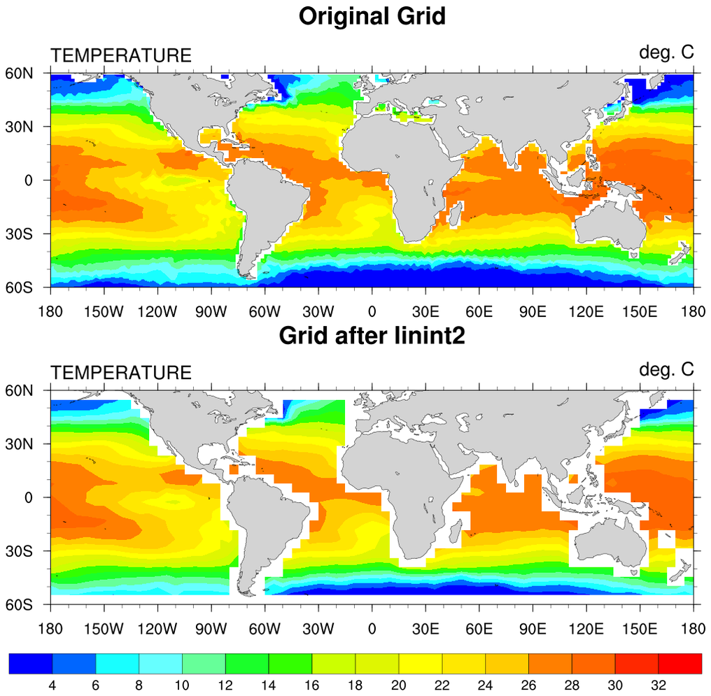
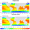 regrid_1.ncl
: An example of using
linint2_Wrap, which interpolates from one grid to
another using bilinear interpolation, and also retains metadata.
 regrid_2.ncl
: An example of using
g2gsh, which interpolates from one gaussian grid to another using
spherical harmonics.
Example: the actual interpolation is conducted using
g2gsh_Wrap,
a wrapper function that will assign all the appropriate meta data,
including the gaussian latitudes, to resulting output.
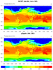
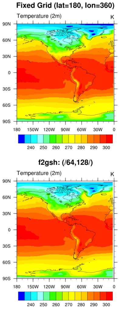
 regrid_3.ncl
: An example of using
g2fsh_Wrap, which interpolates from one gaussian grid to
a fixed grid using spherical harmonics.
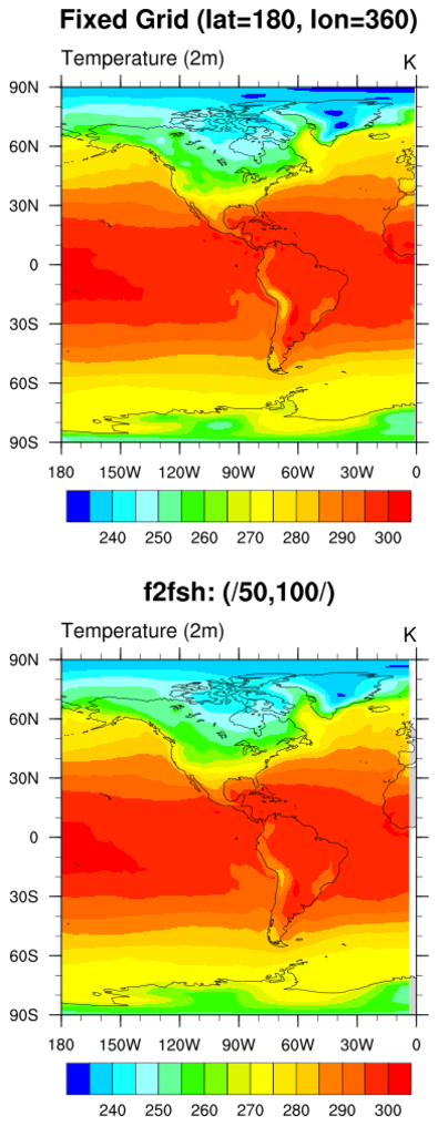
 regrid_4.ncl
: An example of using
f2fsh_Wrap, which interpolates from one fixed grid to another
using spherical harmonics.
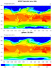
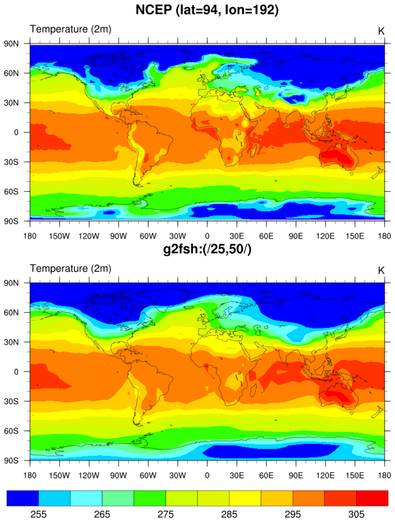
 regrid_5.ncl
: An example of using
f2gsh, which interpolates from a fixed grid to a
gaussian grid using spherical harmonics.
Even though this example uses
f2gsh_Wrap the coordinate
variables could be created manually. See example one for the creation
of the longitude array. The resulting gaussian latitude array can be
created using
latGau.
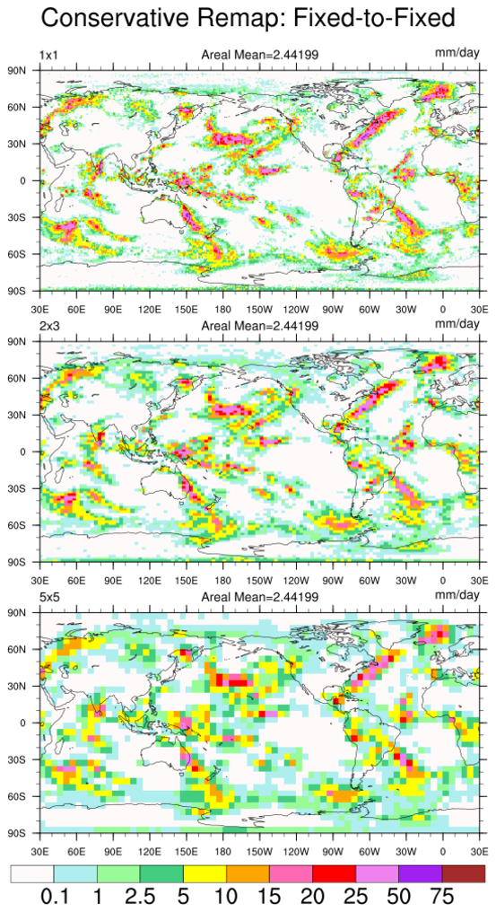
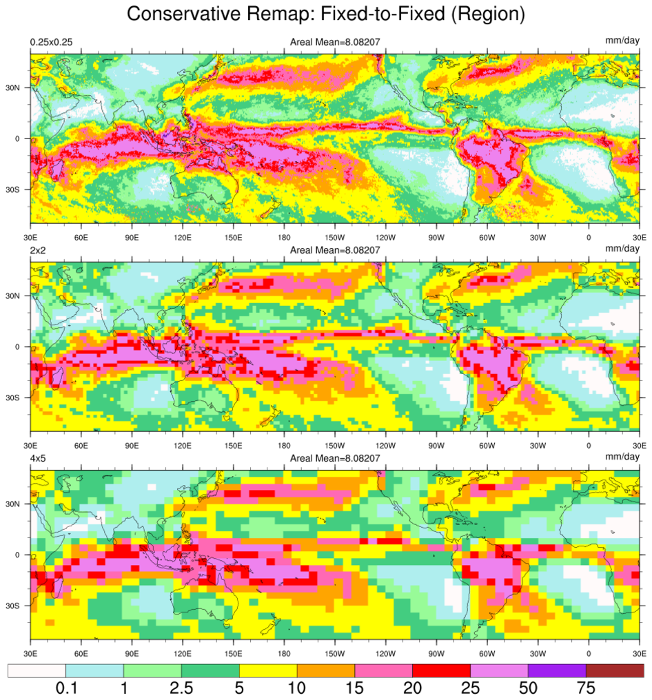
 regrid_6.ncl
: An example of using
area_conserve_remap_Wrap,
to perform an interpolation from a high resolution fixed (regular) grid to
a lower resolution fixed grid. The interpolation is globally conservative.
This function also retains metadata.
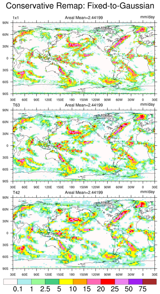
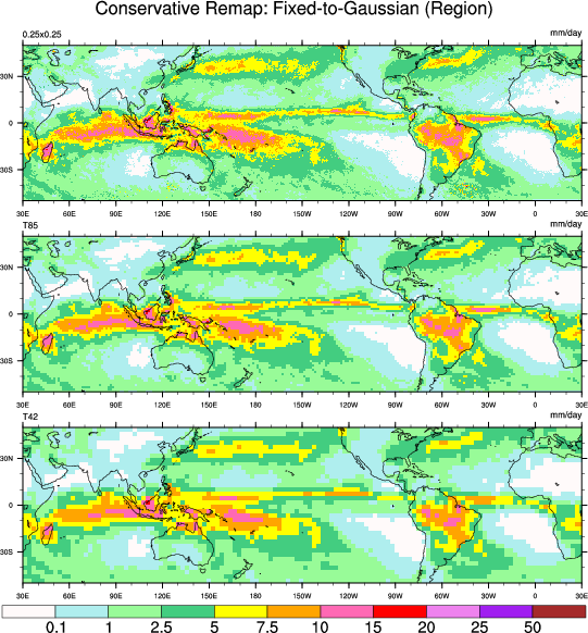
 regrid_7.ncl
: An example of using
area_conserve_remap_Wrap,
to perform an interpolation from a high resolution fixed (regular) grid to
a lower resolution Gaussian grid. The interpolation is globally conservative.
This function also retains metadata.
 regrid_8.ncl
: An example of using
area_conserve_remap_Wrap,
to perform an interpolation from a high resolution Gaussian grid to
a lower resolution Gaussian grid. The interpolation is globally conservative.
This function also retains metadata.
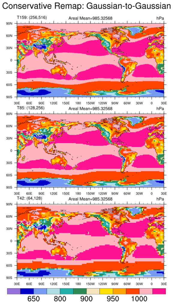
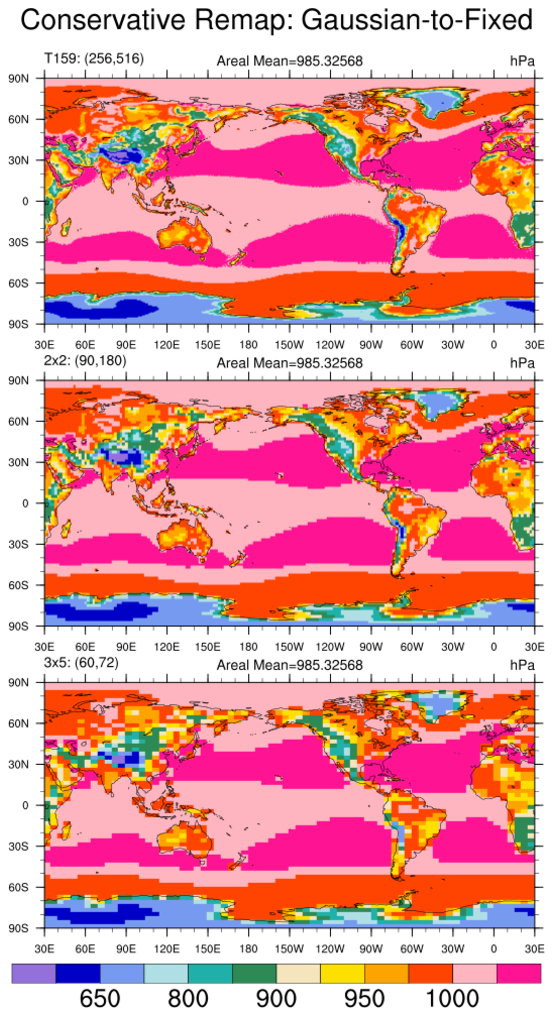
 regrid_9.ncl
: An example of using
area_conserve_remap_Wrap,
to perform an interpolation from a high resolution Gaussian grid to
a lower resolution fixed grid. The interpolation is globally conservative.
This function also retains metadata.
 regrid_10.ncl
: An example of using
area_conserve_remap_Wrap,
to perform an interpolation from a high resolution fixed (regular) grid
with limited latitudinal extent to
a lower resolution fixed grid with approximately the same
latitudinal extent. The interpolation is globally conservative.
This function also retains metadata.
 regrid_11.ncl
: An example of using
area_conserve_remap_Wrap,
to perform an interpolation from a high resolution fixed (regular) grid
with limited latitudinal extent to
a lower resolution gaussian grid with approximately the same
latitudinal extent. The interpolation is
not conservative.
This function also retains metadata.
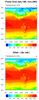
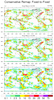
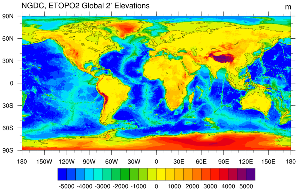
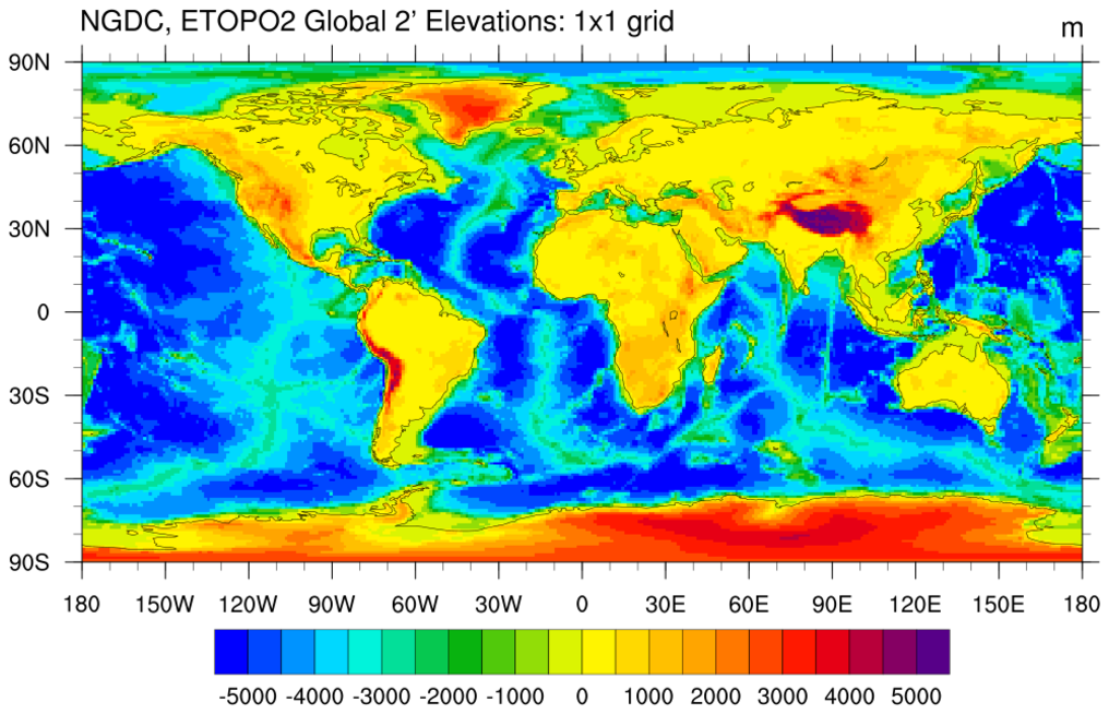
 regrid_12.ncl
: Another simple
example of using
area_conserve_remap_Wrap
to perform an interpolation from a high resolution regular grid
to a lower resolution grid. The variable being regridded is
surface topography [elevation].
This function also retains metadata.
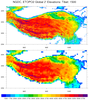
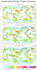
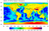
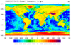
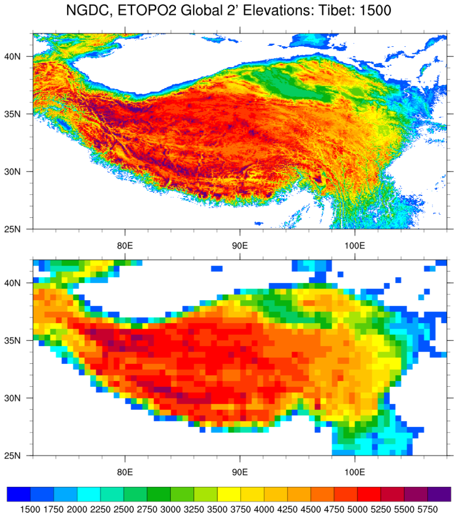
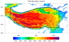 regrid_13.ncl
: Another
example of using
area_conserve_remap_Wrap
to perform an interpolation from a high resolution regular grid
to a lower resolution grid. The variable being regridded is
surface topography [elevation]. It is demonstrated how one
might create a set of lat/lon values that outline Tibet.
The user specified variable "zcrit" can be changed as needed.
The value "zcrit=1500" corresponds to approximately 850 hPa.
"zcrit" values of 2500, 3500 and 4500 would correspond to approxiamtely
750, 650 and 575 hPa, respectively.
This function also retains metadata.
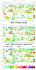
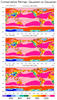
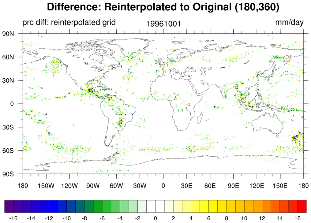
 regrid_14.ncl
: Another
example of using
linint2_Wrap
to perform a bilinear interpolation from a (180,360) regular grid to a
slightly different resolution (192,288) grid. The variable being regridded
is daily precipitation which (generally) has a highly fractal structure.
From point-to-point, the data are not smoothly varying. In fact, they
may well be discontinuous at adjacent grid points. Consider a worst case
scenario of rain rate (mm/day) at 4 adjacent grid points in the source grid (+)
          100           0
           +            +

                 *

           +            +
           0            0
The interpolated value (*) of the target grid (192,288) would (if it was right in the middle) be
* (25) = (100+0+0+0)/4 ; average the source [ + ] gridpoints
This type of thing would occur at all target grid locations.
The only exception would be an instance where the source and target grid locations are identical.
Hence,
in general, source grid maxima & minima are 'lost.'
Now interpolate the target (*) values, which are all weighted averages, back to the original gridded locations (+). In a sense, you are averaging the averages. This reduces the values even more.
**Punch line: interpolation is not reversible.**
Having a smoothly varying variable (eg, temperature, sea-level pressure, ...) minimizes the
effect of interpolation but the issue is still there.
Using ESMF conservative interpolation would preserve the global mean prc in both the original interpolation (MVR grid) and the reinterpolated grid ***BUT*** the price would be a smearing out of the local values. The local differences may be even larger.
The linint2_Wrap function also retains metadata.
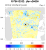
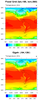
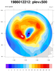
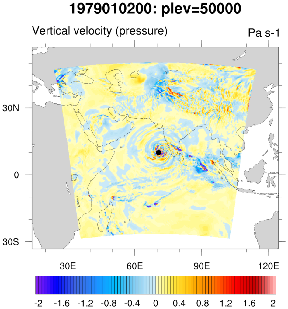
regrid_15.ncl:
Five GRIB2 files are opened via addfiles. The GRIB2 variable containing vertical velocity
("VVEL_P0_L100_GLL0") at 46 pressure levels is imported.
A local library [grid2geocircle.ncl]
contains the rgrid2geolocation interpolation function. The source 'omega' variable is dimensioned:
[forecast_time0 | 5] x [lv_ISBL0 | 46] x [lat_0 | 721] x [lon_0 | 881]
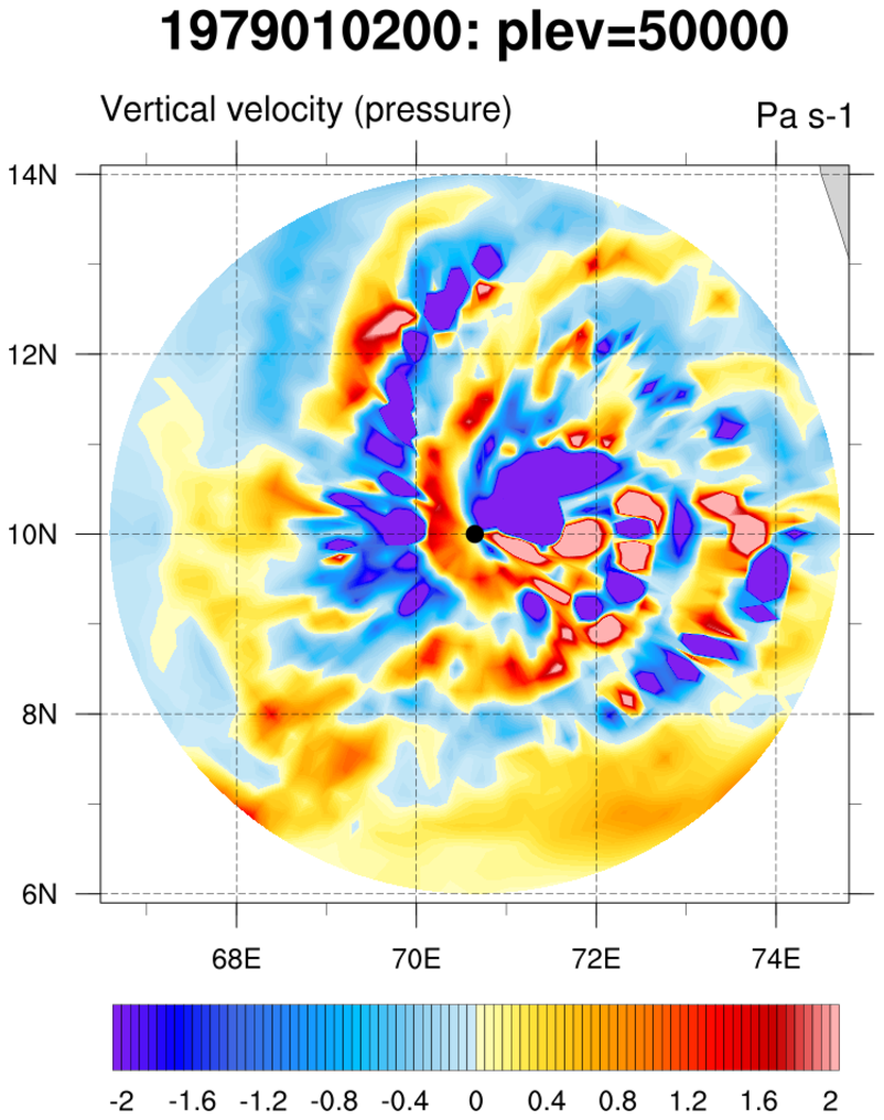
The returned variable is dimensioned:
[forecast_time0 | 5] x [center | 1] x [lv_ISBL0 | 46] x [radius | 17] x [circle | 180]
The radially (azimuthally) averaged variable is dimensioned:
[forecast_time0 | 5] x [center | 1] x [lv_ISBL0 | 46] x [radius | 17]
The data for this example are on a rectilinear grid. Hence, use of the
rgrid2geolocation was appropriate. The library also contains a function appropriate for use with curvilinear grid:
rcm2geolocation.
The regrid_15 also illustrates how a netCDF file may be created.
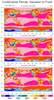
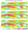
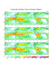
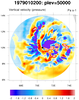
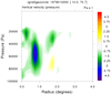
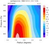
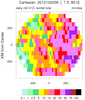
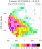
The three figures are:
    (a) original variable at user specified level
    (b) 'radial' interpolated values at locations defined by 'plat' and 'plon'
    (c) 'radial' averaged values at locations each radius
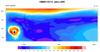
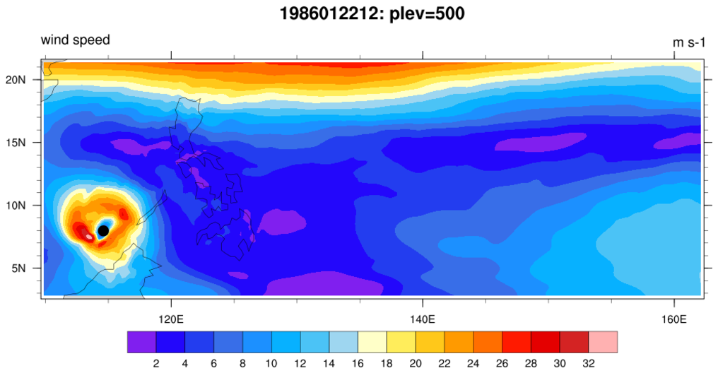
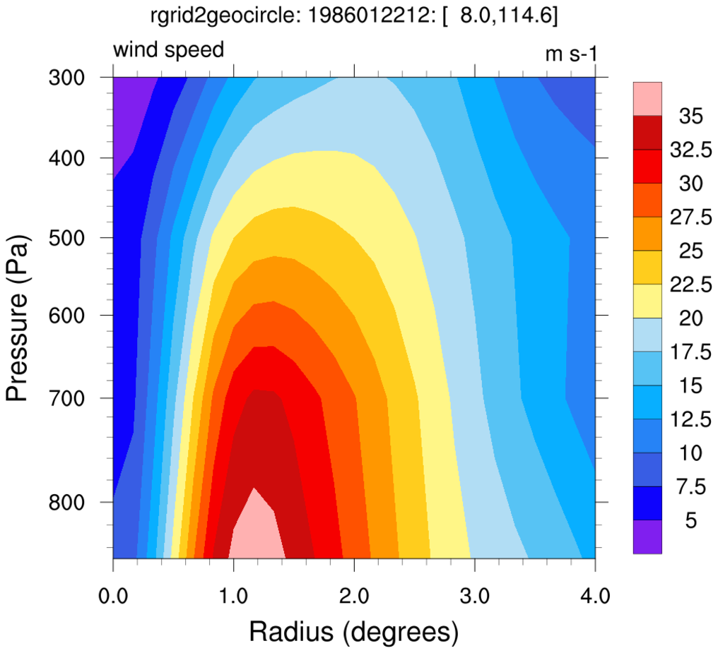
regrid_15_regcm.ncl:
A high resolution RegCM netCDF file is used. The variables are on a rectilinear grid.
A local library [grid2geocircle.ncl]
contains the rgrid2geolocation interpolation function. The source 'ua' and 'va'
variables are used to derive total wind speed. It is dimensioned:
[time | 1] x [plev | 4] x [lat | 84] x [lon | 228]
The returned variable is dimensioned:
[time | 1] x [center | 1] x [plev | 4] x [radius | 25] x [circle | 180]
The radially (azimuthally) averaged variable is dimensioned:
[time | 1] x [center | 1] x [plev | 4] x [radius | 25]
The data for this example are on a rectilinear grid. Hence, use of the
rgrid2geolocation was appropriate. The library also contains a function appropriate for use with curvilinear grid:
rcm2geolocation.
The regrid_15_regcm also illustrates how a netCDF file may be created.
The three figures are:
    (a) original variable at user specified level
    (b) 'radial' interpolated values at locations defined by 'plat' and 'plon'
    (c) 'radial' averaged values at locations each radius
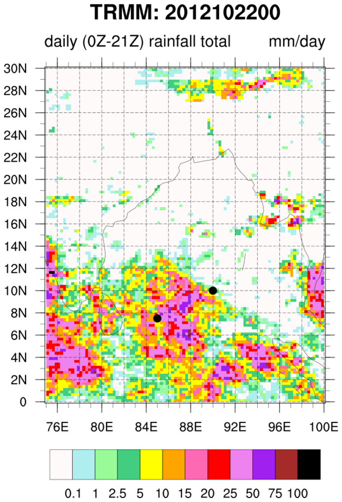
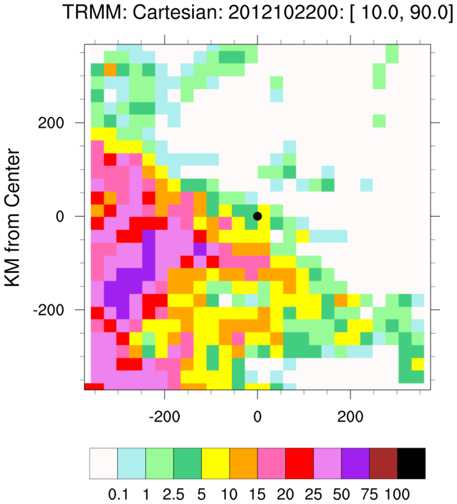
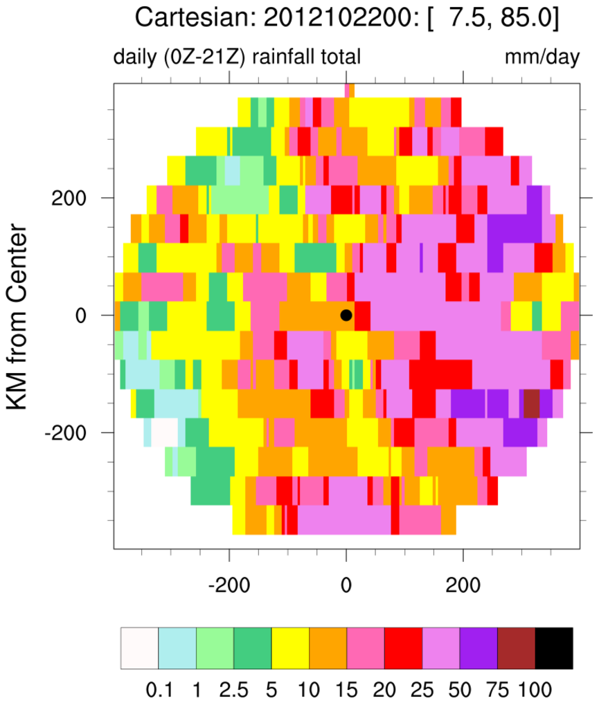
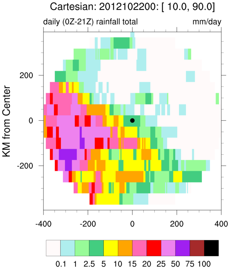
regrid_17.ncl:
Similar to regrid_16:
(a) Read a TRMM netCDF; (b) Specify two locations; (c) Specify distance [km] from the two locations;
(d) Translate the distance in km to degrees; (e) Interpolate the TRMM latitudes and longitudes
to 'geocircles' (aximuthal) locations via a local library
[grid2geocircle.ncl] which
contains the rgrid2geolocation interpolation function.
(f) use css2c to translate the geocircle latitude(s) and longitude(s)
to Cartesian coordinates; (g) center the results about the two locations; (h) plot.
The two figures are:
    (a) Centered cartesian plot for the first location
    (b) Centered cartesian plot for the second location


