NCL Home>
Application examples>
Data sets ||
Data files for some examples
Example pages containing:
tips |
resources |
functions/procedures
NCL: NARR (North American Regional Reanalysis) Data

The NCEP North American Regional Reanalysis (NARR) products are on a
Lambert conformal conic grid (32km) at 29 pressure levels. They were
produced using Eta 32km/45-layer model. The input data includes all
observations used in NCEP/NCAR Global Reanalysis project, and
additional precipitation data, TOVS-1B radiances, profiler data, land
surface and moisture data, etc. The output analyses are 3-hourly with
additional 9 variables in the 3-hour forecasts to reflect
accumulations or averages.
NARR data is distributed on a native lambert conformal grid with 2D latitudes
and longitudes. For a description of native lambert
conformal grids and how to plot them accurately in NCL, click
here, or refer to any of the examples below.
NARR data is available from
NCAR's Research Data Archive
in GRIB format, a subset of NARR data is also available from NOAA's
Earth Systems Research Laboratory (formerly, the Climate
Diagnostics Center [CDC]) in netCDF format. See Example 2.
Important note: in the corners of the images on this page, you
may notice some small slivers of missing data. The original NARR
Eta-12 model grid is regridded to standard NCEP grid 221 for public
distribution, Lambert conformal conic, which you see here.
There is a slight mismatch between the chosen grid boundaries,
resulting in the slivers of missing data. This is discussed on pages
39, 41, 42 of this early Powerpoint summary from NCEP (2005). Page 42
is the picture that speaks a thousand words:
http://www.emc.ncep.noaa.gov/mmb/rreanl/narr.ppt
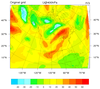 narr_1.ncl
:
This script demonstrates how to quickly read a NARR GRIB
file into NCL, and shows how to plot the data on the NARR native grid.
The file used in the example was obtained from
NCAR's Research Data Archive.
Note that NCL can read GRIB files directly. In addition, NCL provides
additional information [eg, geographical coordinates] that
are not on the original GRIB formatted file. The
ncl_filedump
utility can be used to view any GRIB [nc, hdf-sds, hdf-eos] file as seen via NCL.
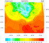 narr_2.ncl
:
This script demonstrates how to read in a NARR netCDF file into NCL. In this case, the data
is stored as 16-bit integers (referred to as type "short"). In general, data of type short
must be transformed prior to calculations and plotting . The contributed function
short2flt may be used to directly read the data. Note
that
short2flt will automatically apply the add_offset and
scale_factor attributes during the conversion from short to float.
NOTE: Some of the NARR
files from NOAA/PSD contain a _FillValue attribute that differs from
the missing_value attribute. This problem has been reported. If
the values look bad, add the following fix suggested by David Allured.
Replace:
x = short2flt( f->air(10,:,:,:) )
with
           xShort  = f->air(10,:,:,:)
           if (isatt(xShort,"_FillValue") .and. isatt(xShort,"missing_value")) then
               if (xShort@_FillValue .ne. xShort@missing_value) then
                   xShort@_FillValue = xShort@missing_value   ; use alt. missing value
               end if                                         ; only if needed
           end if

           x       = short2flt( xShort)
           delete(xShort)                                     ; no longer needed
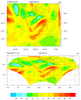 narr_3.ncl
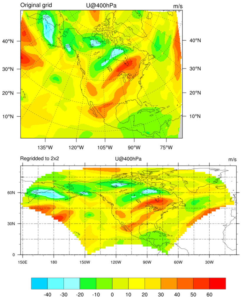
:
This script uses the
triple2grid function to place
values from the NARR Lambert Conformal grid on a 2 degree by 2 degree
grid. Note that no interpolation is done here!
The original grid is plotted in the top panel, while the regridded
data is shown in the bottom panel. The sample script outputs a netCDF
file containing the interpolated 2x2 grid. An
ncl_filedump of the
netCDF file is here.
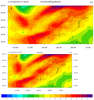 narr_4.ncl
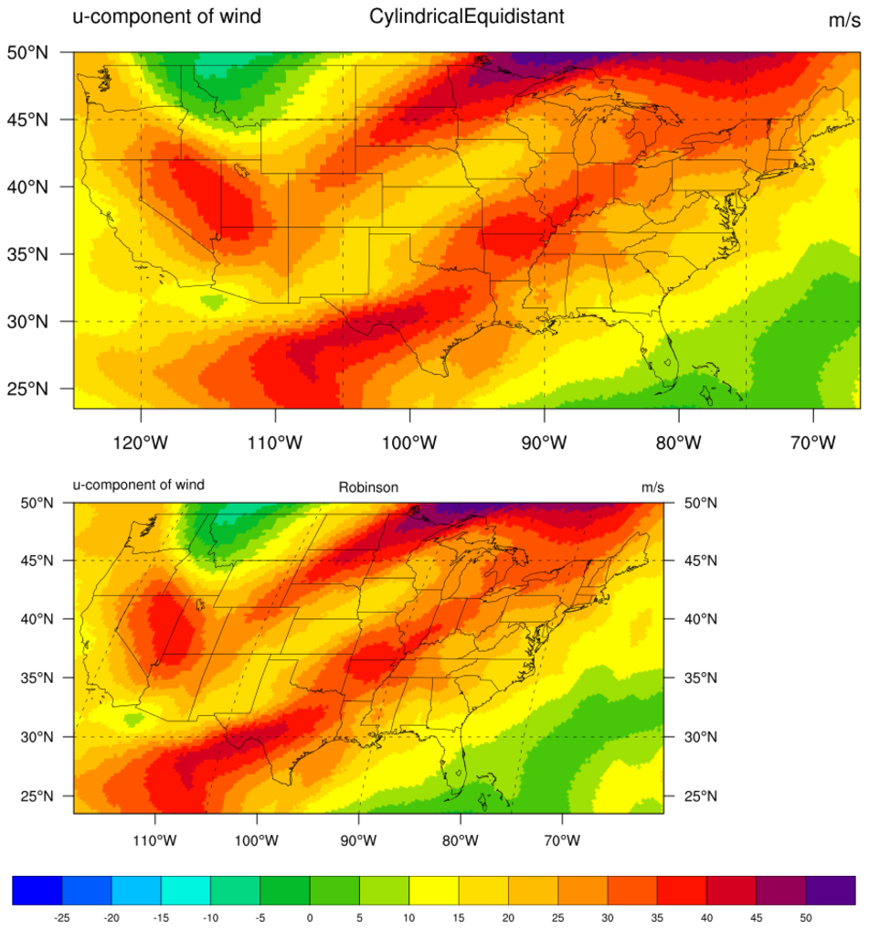
:
This script uses the same files used in Example 1. The data
are on a Lambert Conformal projection. The narr_4.ncl script
plots the region of the lower 48 United States using two different
map projections: Cylindrical Equidistant and Robinson.
Further, the
mpLimitMode= "LatLon" is used to manually
set the appropriate limits for each projection.
 narr_5.ncl
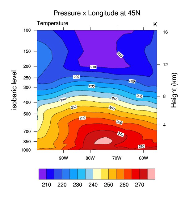
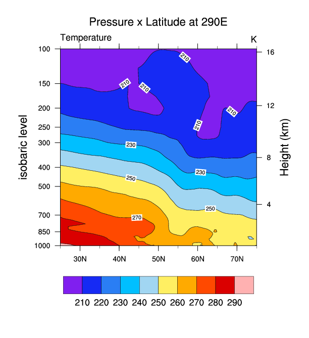
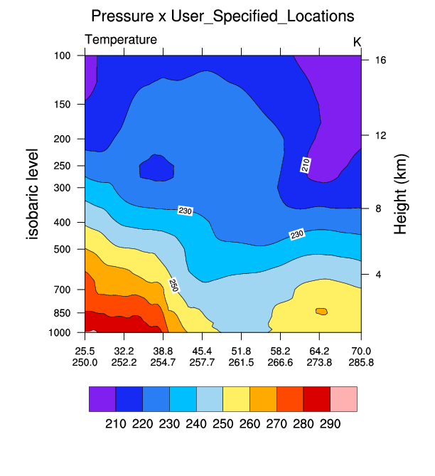
:
This script uses an ESMF generated weight file
(see
ESMF example 30) to efficiently regrid a
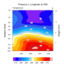
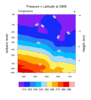
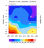
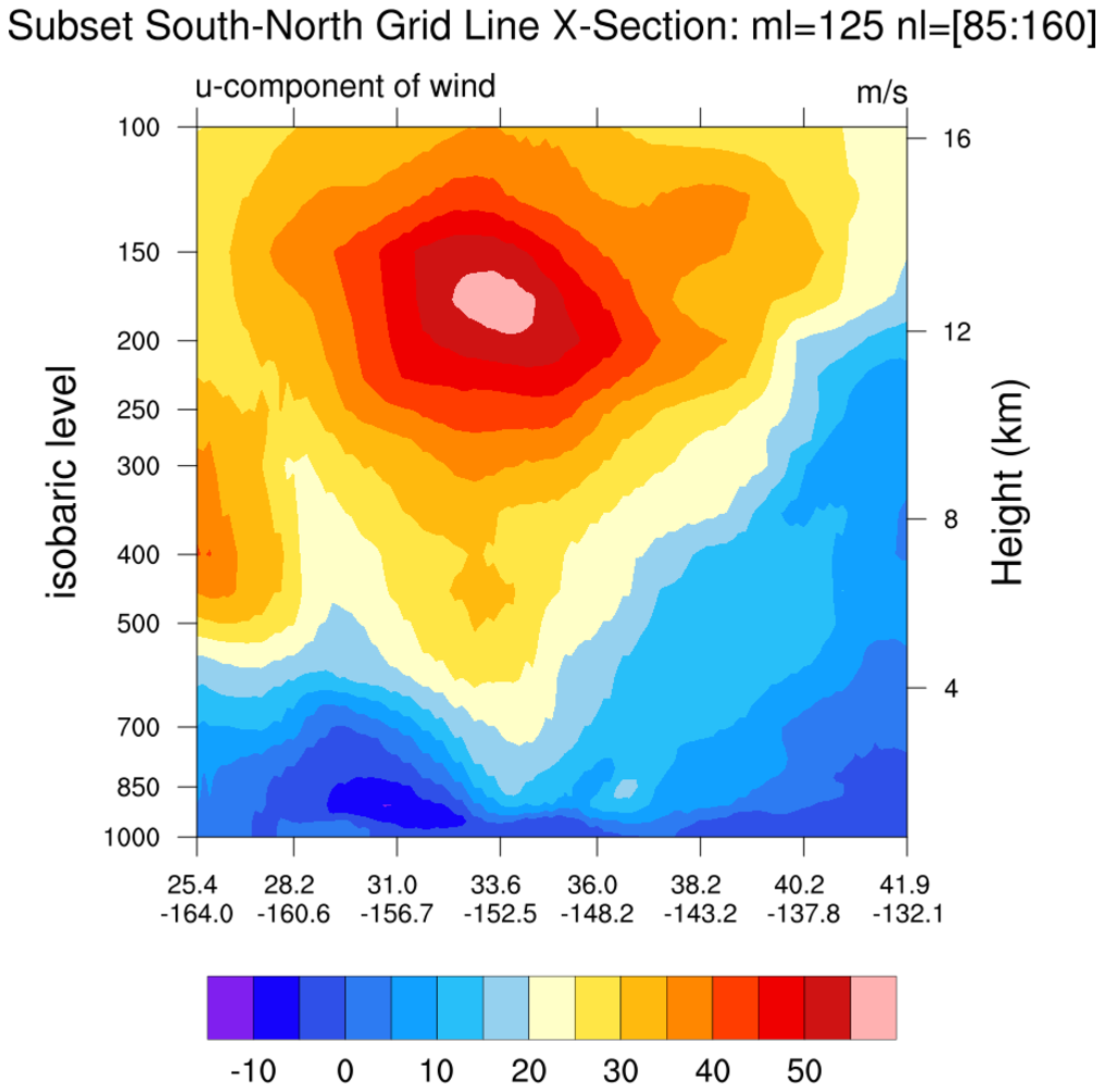
source NARR curvilinear grid to a rectilinear grid. Then three cross sections are plotted:
(a) pressure x longitude; (b) pressure x latitude; and, (c) pressure x user_specfiied_set_of_points.
For this example the user specified latitude/longitude locations lie along a great circle path
between two user specified locations (see
gc_latlon). They could be
latitude/longitude locations along a (say) cold front.
ESMF example 30
was run twice: bilinear and conservative interpolation. Bilinear interpolation
would generally be appropriate for any reasonably smooth variable. Conservation interpolation
would be recommended for interpolating flux quantities and variables that can be fractal (eg precipitation).
narr_7.ncl:
ncl-talk question: How can I interpolate NARR data to particular points
in space at specific heights (lat_pt, lon_pt, height)?
This example creates a function to perform the necessary tasks:
(i) vertical interpolation to specified height levels;
(ii) interpolate from a NARR curvilinear grid to a rectilinear grid; and
(iii) use linint2_points_Wrap to interpolate to specified locations.
The interpolated variable at 3 heights and 2 locations (pts) looks like:
      Variable: x_pts
      Number of Dimensions: 3
      Dimensions and sizes:	[initial_time0_hours | 1] x [hgt | 3] x [pts | 2]
      Coordinates:
                  initial_time0_hours: [1852632..1852632]
                  hgt: [375..1865]
                  pts: [0..1]
      Number Of Attributes: 16
        ycoord :	(  22.3, 47.8 )   <=== interpolated locations
        xcoord :	(-135.3, 157.2)   <===      "          "
      [SNIP]
The values are:
	 nt=0  hgt=375

	 22.30  -135.30   289.85
	 47.80  157.20   279.61
	 ----------------------

	 nt=0  hgt=1340

	 22.30  -135.30   288.19
	 47.80  157.20   277.27
	 ----------------------
	 nt=0  hgt=1865

	 22.30  -135.30   284.37
	 47.80  157.20   274.01

