NCL Home>
Application examples>
Maps and map projections ||
Data files for some examples
Example pages containing:
tips |
resources |
functions/procedures
NCL Graphics: Lambert Conformal Native Grid Projections
WARNING
Is your data on a native grid? A native grid is a model that was
designed from the beginning with a particular map projection. In order
to plot the data exactly as the designers planned, we do not want to
transform the data to a projection, but simply plot it. This is the
essence of the examples on this page.
Just because your data has 2D lat/lon arrays, does not make it a
native grid. Native grids are plotted differently than other data
with 2D coordinates.
In all cases, you MUST use the
mpLimitMode="Corners" method to
specify the grid. Other methods will
result in an incorrect mismatch between the data and the map.
Additionally, you must set
tfDoNDCOverlay = True so that
the data is not transformed to the
projection, but is simply placed there since it is already on a
projection.
pmTickMarkDisplayMode =
"Always" turns on nicer tickmark labels.
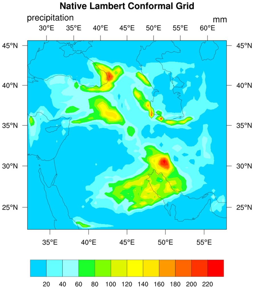
 lcnative_1.ncl
: An example of
plotting
netCDF data that is on a Lambert Conformal
native grid. See the next section for an example of plotting this
data on a cylindrical equidistant map projection.
netCDF files may or may not contain the parallel information
needed to plot the grid correctly. Grids on GRIB files
(see example 4) contain this information.
mpProjection =
"LambertConformal", sets the projection.
The three pieces of information that are required for this projection
(with example values) are:
mpLambertParallel1F = 36.
mpLambertParallel2F = 55.
mpLambertMeridianF = 45.
The problem with Lambert grids is they are are sometimes described
by a meridian, parallel and a delta X and delta Y in meters at the
intersection of the meridian and top parallel. It can be VERY
difficult to come up with corner points when this method is used.
A note about this particular example: Since no information was able
on the grid, we assumed that the lat, lon arrays started in the lower
left corner. Another RCM-2 user found a different array order, which
resulted in the following "corners" selections:
mpLeftCornerLatF = lat2d(nlat-1,0)
mpLeftCornerLonF = lon2d(nlat-1,0)
mpRightCornerLatF = lat2d(0,nlon-1)
mpRightCornerLonF = lon2d(0,nlon-1)
A Python version of this projection is available here.
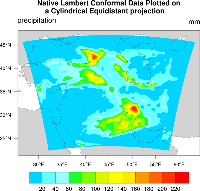
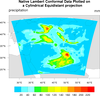 lcnative_latlon_1.ncl
:
This example plots the same data as the previous "lcnative_1.ncl"
example, except it projects it onto the default cylindrical
equidistant map projection.
The special "lat2d" and "lon2d" attributes are attached to the
data, so the plotting routine knows what the lat/lon values are.
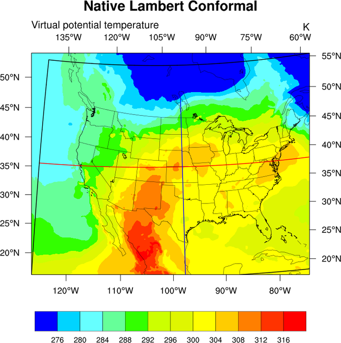
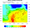 lcnative_2.ncl
: Native lambert
conformal grid from a GRIB file. GRIB files contain the parallel
information, and NCL automatically reads these values in and assigns
them as attributes to the lat2d array.
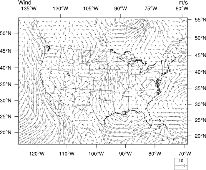
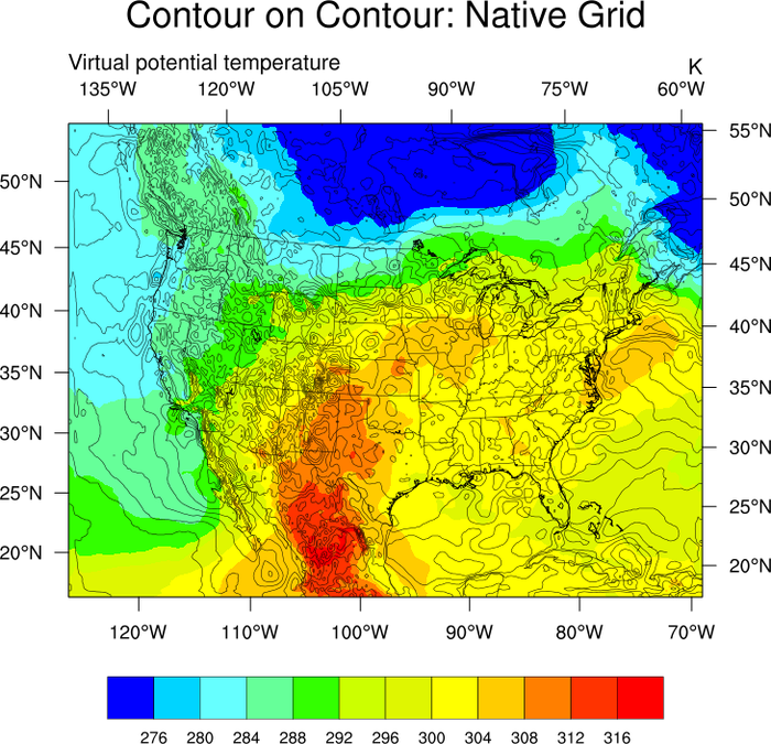
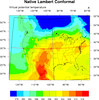 lcnative_3.ncl
: There are times
when you may not know the appropriate parallels for your native
lambert conformal grid. This examples demonstrates one way to find
out.
- As a first guess, start with the parallels in the center of the grid.
- look at the lines plotted on the map (see below). You know the
projection is correct when the red and blue lines form a right angle
between themselves and the border.
-
Iterate as necessary to get the closest solution. Your best bet of course
is to get this info from the model itself.

