       lat2d     = f->TLAT
       lon2d     = f->TLONG
       t@lon2d   = lon2d
       t@lat2d   = lat2d
NCL Home>
Application examples>
Models ||
Data files for some examples
 popscal_2.ncl: Shades values less
than five.
popscal_2.ncl: Shades values less
than five.
The gsn_contour_shade function fills contours less than/greater than or equal to the numeric arguments passed to it. Whether or not to fill with color or pattern, and which color/pattern to fill high/middle/low ranges with, are determined by attributes attached to the "opt" argument. Detailed information about gsn_contour_shade can be found on the function's documentation page on the NCL website.
There are many other contour effects that you can use for your own contour plots.
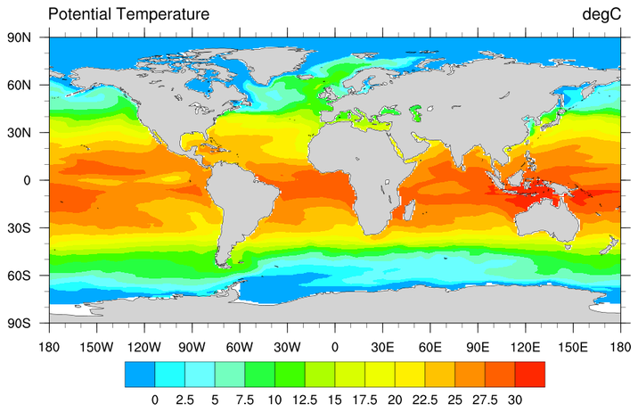
 popscal_3.ncl: Creates a color plot
The color fill example page is a good resource for learning about color plots.
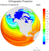 popscal_4.ncl: Shows how to draw
vectors over scalars on another projection.
You are not limited to cylindrical equidistant projections. There are
several projections to choose from.
popscal_4.ncl: Shows how to draw
vectors over scalars on another projection.
You are not limited to cylindrical equidistant projections. There are
several projections to choose from.
This is an orthographic projection. If you wish to view a CE projection, gsn_csm_vector_scalar_map_ce is the function to use: Example.
Example pages containing:
tips |
resources |
functions/procedures
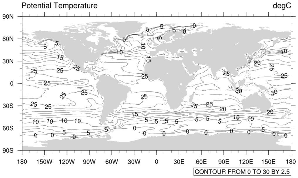
NCL Graphics: POP Scalars
POP data that have 2D lat/lon coordinates
can be plotted directly in physical space. To do this, simply read in
the two dimensional arrays containing the grid point coordinates and
assign the arrays to the variable to be plotted as attributes with
the specific names lon2d and lat2d:
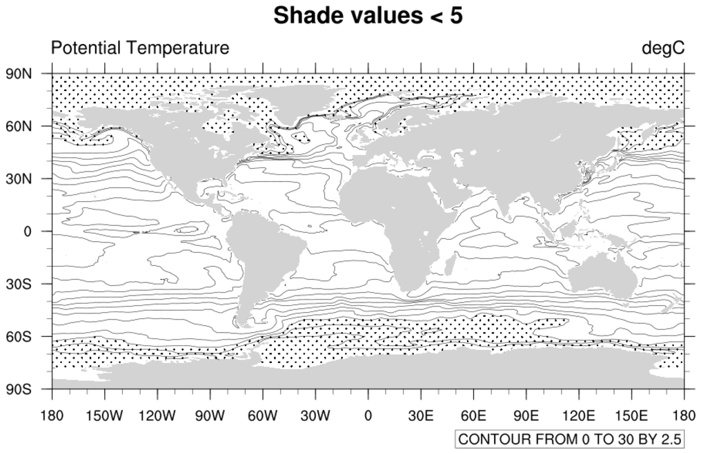 popscal_2.ncl: Shades values less
than five.
popscal_2.ncl: Shades values less
than five.
The gsn_contour_shade function fills contours less than/greater than or equal to the numeric arguments passed to it. Whether or not to fill with color or pattern, and which color/pattern to fill high/middle/low ranges with, are determined by attributes attached to the "opt" argument. Detailed information about gsn_contour_shade can be found on the function's documentation page on the NCL website.
There are many other contour effects that you can use for your own contour plots.
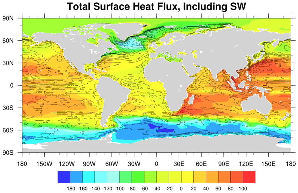
popscal_3.ncl: Creates a color plot
The color fill example page is a good resource for learning about color plots.
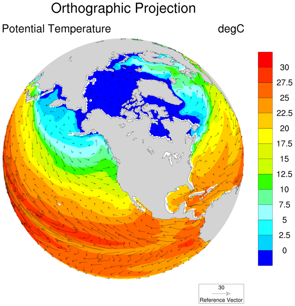 popscal_4.ncl: Shows how to draw
vectors over scalars on another projection.
You are not limited to cylindrical equidistant projections. There are
several projections to choose from.
popscal_4.ncl: Shows how to draw
vectors over scalars on another projection.
You are not limited to cylindrical equidistant projections. There are
several projections to choose from.
This is an orthographic projection. If you wish to view a CE projection, gsn_csm_vector_scalar_map_ce is the function to use: Example.