GSUN > Examples > 1 | 2 | 3 | 4 | 5 | 6 | 7 | 8 | 9 | 10 | 11
Example 6 - vector plots over maps
This example reads in some netCDF files and creates three vector plots over different map projections. Resources are used to change aspects of both the vectors and the maps.To run this example, you must download the following file:
gsun06n.ncland then type:
ncl gsun06n.ncl
Output from example 6
| Frame 1 | Frame 2 | Frame 3 |
|---|---|---|
| 
| 
|
(Click on any frame to see it enlarged.)
NCL code for example 6
  1. load "$NCARG_ROOT/lib/ncarg/nclscripts/csm/gsn_code.ncl"
  2.
  3. begin
  4.   dir = ncargpath("data")
  5.   uf = addfile(dir+"/cdf/Ustorm.cdf","r")  ; Open three netCDF files.
  6.   vf = addfile(dir+"/cdf/Vstorm.cdf","r")
  7.   tf = addfile(dir+"/cdf/Tstorm.cdf","r")
  8.
  9.   u   = uf->u(0,:,:)   ; Get u, v, lat, lon data.
 10.   v   = vf->v(0,:,:)
 11.   lat = uf->u&lat
 12.   lon = uf->u&lon
 13.
 14.   wks = gsn_open_wks("x11","gsun06n") ; Open a workstation.
 15.
 16. ;----------- Begin first plot -----------------------------------------
 17.
 18.   resources = True
 19.
 20.   nlon = dimsizes(lon)
 21.   nlat = dimsizes(lat)
 22.   resources@vfXCStartV  = lon(0)      ; Define lat/lon corners
 23.   resources@vfXCEndV    = lon(nlon-1) ; for vector plot.
 24.   resources@vfYCStartV  = lat(0)
 25.   resources@vfYCEndV    = lat(nlat-1)
 26.
 27.   map = gsn_vector_map(wks,u,v,resources)  ; Draw a vector plot of u and v
 28.                                            ; over a map.
 29. ;----------- Begin second plot -----------------------------------------
 30.
 31.   resources@mpLimitMode       = "Corners"  ; Zoom in on the plot area.
 32.   resources@mpLeftCornerLonF  = lon(0)
 33.   resources@mpRightCornerLonF = lon(nlon-1)
 34.   resources@mpLeftCornerLatF  = lat(0)
 35.   resources@mpRightCornerLatF = lat(nlat-1)
 36.
 37.   resources@mpPerimOn         =   True    ; Turn on map perimeter.
 38.
 39.   resources@vpXF      = 0.1   ; Increase size and change location
 40.   resources@vpYF      = 0.92  ; of vector plot.
 41.   resources@vpWidthF  = 0.75
 42.   resources@vpHeightF = 0.75
 43.
 44.   resources@vcMonoLineArrowColor = False  ; Draw vectors in color.
 45.   resources@vcMinFracLengthF     = 0.33   ; Increase length of
 46.   resources@vcMinMagnitudeF      = 0.001  ; vectors.
 47.   resources@vcRefLengthF         = 0.045
 48.   resources@vcRefMagnitudeF      = 20.0
 49.
 50.   map = gsn_vector_map(wks,u,v,resources)  ; Draw a vector plot.
 51.
 52. ;----------- Begin third plot -----------------------------------------
 53.
 54.   temp  = (tf->t(0,:,:)-273.15)*9.0/5.0+32.0 ; Read in temp data and
 55.                                              ; convert from K to F.
 56.
 57.   cmap = (/(/1.00, 1.00, 1.00/), (/0.00, 0.00, 0.00/), (/.560, .500, .700/), \
 58.            (/.300, .300, .700/), (/.100, .100, .700/), (/.000, .100, .700/), \
 59.            (/.000, .300, .700/), (/.000, .500, .500/), (/.000, .700, .100/), \
 60.            (/.060, .680, .000/), (/.550, .550, .000/), (/.570, .420, .000/), \
 61.            (/.700, .285, .000/), (/.700, .180, .000/), (/.870, .050, .000/), \
 62.            (/1.00, .000, .000/), (/.700, .700, .700/)/)
 63.
 64.   gsn_define_colormap(wks, cmap)  ; Define a new color map.
 65.
 66.   resources@mpProjection = "Mercator"  ; Change the map projection.
 67.   resources@mpCenterLonF = -100.0
 68.   resources@mpCenterLatF =   40.0
 69.
 70.   resources@mpLimitMode  = "LatLon"  ; Change the area of the map
 71.   resources@mpMinLatF    =  18.0     ; viewed.
 72.   resources@mpMaxLatF    =  65.0
 73.   resources@mpMinLonF    = -128.
 74.   resources@mpMaxLonF    = -58.
 75.
 76.   resources@mpFillOn               = True  ; Turn on map fill.
 77.   resources@mpLandFillColor        = 16    ; Change land color to grey.
 78.   resources@mpOceanFillColor       = -1    ; Change oceans and inland
 79.   resources@mpInlandWaterFillColor = -1    ; waters to transparent.
 80.
 81.   resources@mpGridMaskMode         = "MaskNotOcean"  ; Draw grid over ocean.
 82.   resources@mpGridLineDashPattern  = 2
 83.
 84.   resources@vcFillArrowsOn           = True  ; Fill the vector arrows
 85.   resources@vcMonoFillArrowFillColor = False ; using multiple colors.
 86.   resources@vcFillArrowEdgeColor     = 1     ; Draw the edges in black.
 87.
 88.   resources@tiMainString      = ":F25:Wind velocity vectors"  ; Title
 89.   resources@tiMainFontHeightF = 0.03
 90.
 91.   resources@pmLabelBarDisplayMode  = "Always"     ; Turn on a label bar.
 92.   resources@pmLabelBarSide         = "Bottom"     ; Change orientation
 93.   resources@lbOrientation          = "Horizontal" ; of label bar.
 94.   resources@lbPerimOn              = False        ; Turn off perimeter.
 95.   resources@lbTitleString          = "TEMPERATURE (:S:o:N:F)" ; Title for
 96.   resources@lbTitleFont            = 25                       ; label bar.
 97.
 98.   resources@mpOutlineBoundarySets = "GeophysicalAndUSStates"
 99.
100.   map = gsn_vector_scalar_map(wks,u(::2,::2),v(::2,::2),temp(::2,::2),resources)
101.
102.   delete(resources) ; Clean up.
103.   delete(map)
104.   delete(u)
105.   delete(v)
106.   delete(temp)
107. end
Explanation of example 6
Lines 4-7:
  dir = ncargpath("data")
  uf = addfile(dir+"/cdf/Ustorm.cdf","r")
  vf = addfile(dir+"/cdf/Vstorm.cdf","r")
  tf = addfile(dir+"/cdf/Tstorm.cdf","r")
Open three netCDF files containing storm data; uf, vf, and tf are references to the files specified in the addfile function.
  u   = uf->u(0,:,:)
  v   = vf->v(0,:,:)
  lat = uf->u&lat
  lon = uf->u&lon
Read the variables u and v and the coordinate variables lat and lon from two of the netCDF file references, uf and vf and store them to local NCL variables.
uf->u and vf->v are 3-dimensional arrays (of the same size) of wind velocity vector data, where the first dimension represents time, the second dimension represents latitude, and the third dimension represents longitude (verify this with print(getfilevardims(uf,"u"))). By using the syntax (0,:,:), you are selecting the vector field for the full latitude/longitude range for the first time step only.
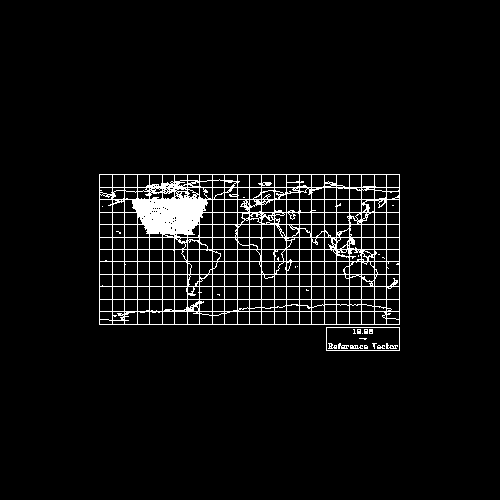
;----------- Begin first plot -----------------------------------------Draw a vector plot over a map, using the default map projection (cylindrical equidistant). The only resources set for this plot are for determining where on the map the vector plot should be overlaid.
  nlon = dimsizes(lon)
  nlat = dimsizes(lat)
  resources@vfXCStartV  = lon(0)
  resources@vfXCEndV    = lon(nlon-1)
  resources@vfYCStartV  = lat(0)
  resources@vfYCEndV    = lat(nlat-1)
Set some VectorField resources to define the two corners of the latitude/longitude rectangle to overlay the vector plot on. A more detailed description of overlaying plots on a map plot is in example 5, which explains the overlay process of a contour plot on a map using ScalarField resources. The same explanation applies to the VectorField resources used here. The VectorField resources themselves are described in more detail in example 3.
map = gsn_vector_map(wks,u,v,resources)Create and draw a vector plot of the u and v variables over a map. The default map projection is cylindrical equidistant. The first argument of the gsn_vector_map function is the workstation variable returned from the previous call to gsn_open_wks. The next two arguments represent the 2-dimensional vector field to be plotted (they must have the same dimensions and can be of type float, double, or integer). The last argument is a logical value indicating whether you have set any resources.
Note that the vector plot covers only a small area of the map. This is because the latitude values you specified in lines 20-25 only go from 20 to 60, and the longitude values go from -140 to -52.5 (you can verify this by using print to print these values out). These latitude/longitude values roughly cover the area which is the United States, so this is where you'll see the vector plot overlaid.
As described in example 5 for gsn_contour_map, the gsn_vector_map function creates two plots, the vector plot and the map plot. The map plot is what's returned from the function, and the vector plot is returned as an attribute of the map plot called "vector."
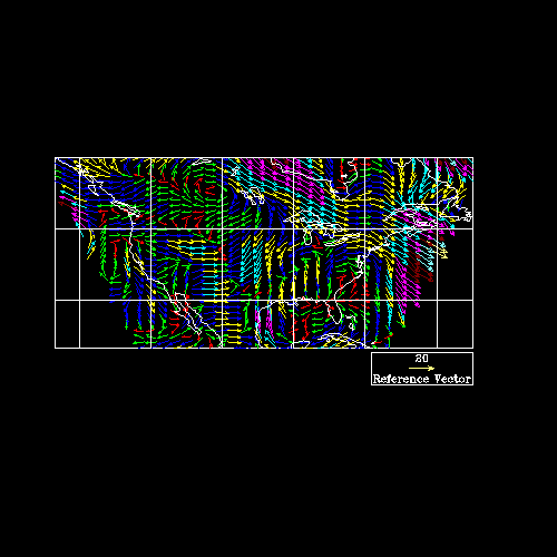
;----------- Begin second plot -----------------------------------------Zoom in on the area of the map that contains the vector plot, draw the vectors in color and make them larger, and increase the size of the plot within the viewport.
  resources@mpLimitMode       = "Corners"
  resources@mpLeftCornerLonF  = lon(0)
  resources@mpRightCornerLonF = lon(nlon-1)
  resources@mpLeftCornerLatF  = lat(0)
  resources@mpRightCornerLatF = lat(nlat-1)
Set some resources to zoom in on the area of the map where the vectors are concentrated. Use the same bounds that you used to define the area that the vector plot is overlaid on.
  resources@vpXF      = 0.1
  resources@vpYF      = 0.92
  resources@vpWidthF  = 0.75
  resources@vpHeightF = 0.75
Set some resources to change the size and position of the plot you want to draw in the viewport. The viewport is discussed in more detail in example 5.
  resources@vcMonoLineArrowColor = False
  resources@vcMinFracLengthF     = 0.33
  resources@vcMinMagnitudeF      = 0.001
  resources@vcRefLengthF         = 0.045
  resources@vcRefMagnitudeF      = 20.0
Set some resources to draw the vectors in color and to increase their lengths. The above resources are described in more detail in example 3. The default color map is used in this case.
map = gsn_vector_map(wks,u,v,resources)Create and draw a vector plot of u and v over a map. This time you should be able to see the vector plot better since you zoomed in on the area of the map containing the vectors.
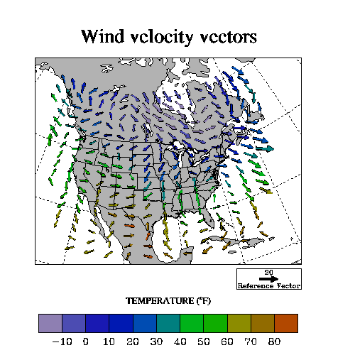
;----------- Begin third plot -----------------------------------------Create your own color map, draw filled vectors instead of line vectors, color the vectors according to a temperature scalar field, change the map projection, fill land in gray, mask the map grid over land, thin the vectors, and draw a label bar at the bottom of the plot.
temp = (tf->t(0,:,:)-273.15)*9.0/5.0+32.0Select the first time step of the temperature data in one of the netCDF files that you opened earlier, convert the values from Kelvin to Fahrenheit, and store the data to a local NCL variable called temp.
  cmap = (/(/1.00, 1.00, 1.00/), (/0.00, 0.00, 0.00/), (/.560, .500, .700/), \
           (/.300, .300, .700/), (/.100, .100, .700/), (/.000, .100, .700/), \
           (/.000, .300, .700/), (/.000, .500, .500/), (/.000, .700, .100/), \
           (/.060, .680, .000/), (/.550, .550, .000/), (/.570, .420, .000/), \
           (/.700, .285, .000/), (/.700, .180, .000/), (/.870, .050, .000/), \
           (/1.00, .000, .000/), (/.700, .700, .700/)/)

  gsn_define_colormap(wks, cmap)
Define a color map with 17 entries having a white background and a
black foreground. Details on creating your own color map are covered
in example
2.
  resources@mpProjection = "Mercator"
  resources@mpCenterLonF = -100.0
  resources@mpCenterLatF =   40.0
Change the map projection to "Mercator" and change the center longitude and latitude values to be the approximate center of the latitude/longitude rectangle you're about to define when you set the mpLimitMode resource.
  resources@mpLimitMode  = "LatLon"
  resources@mpMinLatF    =  18.0
  resources@mpMaxLatF    =  65.0
  resources@mpMinLonF    = -128.
  resources@mpMaxLonF    = -58.
Change the mode for zooming in on the map projection to "LatLon". When mpLimitMode is set to this string, the resources mpMinLatF, mpMaxLatF, mpMinLonF, and mpMaxLonF are used to determine the limits of the maximum viewable portion of the map in latitude/longitude coordinates.
  resources@mpFillOn               = True
  resources@mpLandFillColor        = 16
  resources@mpOceanFillColor       = -1
  resources@mpInlandWaterFillColor = -1
Turn on the filling of map geographical areas, and fill the land gray and the oceans and inland water transparent. Note that this method is different that the one used in example 5 where the map areas you wanted to fill were specified with the resource mpFillColors. Either method could have been used in this case, since you filling the same types of areas.
  resources@mpGridMaskMode         = "MaskNotOcean"
  resources@mpGridLineDashPattern  = 2
Draw the map latitude/longitude grid lines over the ocean only, and use a dashed line to draw the grid (the default is a solid line).
  resources@vcFillArrowsOn           = True
  resources@vcMonoFillArrowFillColor = False
  resources@vcFillArrowEdgeColor     = 1
Set some resources to indicate that you want multi-colored filled vector arrows and the edges of the arrows drawn in the foreground color. By default, the edges of the arrows are drawn in the background color.
  resources@pmLabelBarDisplayMode  = "Always"
  resources@pmLabelBarSide         = "Bottom"
  resources@lbOrientation          = "Horizontal"
  resources@lbPerimOn              = False
  resources@lbTitleString          = "TEMPERATURE (:S:o:N:F)"
  resources@lbTitleFont            = 25
Turn on the drawing of a label bar, title it, and put it at the bottom of the plot. The text function code ":S:o:N:F" draws an "o" as a superscript character before the letter "F", to indicate "degrees Fahrenheit."
resources@mpOutlineBoundarySets = "GeophysicalAndUSStates"The mpOutlineBoundarySets resource allows you to indicate what kind of map outlines to draw. Using a value of "GeophysicalAndUSStates" draws outlines of all global geophysical features and also U.S. States and inland water features. The default of mpOutlineBoundarySets is "Geophysical."
map = gsn_vector_scalar_map(wks,u(::2,::2),v(::2,::2),temp(::2,::2),resources)Use the gsn_vector_scalar_map function to draw a vector plot over a map and color the vectors according to the scalar field temp. The gsn_vector_scalar_map function is the same as the gsn_vector_map function, only it has a scalar field as an additional argument (the fourth argument). The scalar field must be the same dimensions as the U and V arrays.
In the call to gsn_vector_scalar_map, the syntax "(::2)" is being used to "thin" the vectors; that is, only every other data point is passed on to the plotting function.