GSUN > Examples > 1 | 2 | 3 | 4 | 5 | 6 | 7 | 8 | 9 | 10 | 11
Example 9 - animated contours over a map
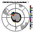
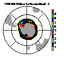
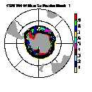
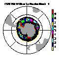
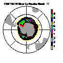
This example reads data from a netCDF file and creates a 12-frame animation of contours over a polar stereographic map projection. This example also uses a resource file and shows how to create a function in an NCL script.To run this example, you must download the following files:
gsun09n.ncland then type:
gsun09n.res
ncl gsun09n.ncl
Selected output from example 9
| Frame 3 | Frame 5 | Frame 7 | Frame 9 | Frame 11 |
|---|
(Click on any frame to see it enlarged or view the 12-frame animation.)
NCL code for example 9
  1. load "$NCARG_ROOT/lib/ncarg/nclscripts/csm/gsn_code.ncl"
  2.
  3. function addcyclic(data[*][*]:float)
  4. ;
  5. ; Add a cyclic point in "x" to a 2D array
  6. ; for a lat/lon plot "x"  corresponds to "lon"
  7. ;                    "ny" corresponds to "nlat"
  8. ;                    "mx" corresponds to "mlon"
  9. local dims, newdata, ny, mx, mx1
 10. begin
 11.     dims    = dimsizes(data)
 12.     ny      = dims(0)
 13.     mx      = dims(1)
 14.     mx1     = mx+1
 15.
 16.     newdata = new((/ny  ,mx1/),float)
 17.
 18.     newdata(:,0:mx-1) = data             ; pass everything
 19.     newdata(:,mx)     = (/ data(:,0) /)  ; value only
 20.
 21.     if((.not.ismissing(newdata!1)) .and. iscoord(data,newdata!1)) then
 22.         newdata&$newdata!1$(mx) = newdata&$newdata!1$(0) + 360.0
 23.     end if
 24.
 25.     return(newdata)
 26. end
 27.
 28. begin
 29.
 30.   file1 = ncargpath("data") + "/cdf/fice.nc"
 31.
 32.   ice1 = addfile(file1,"r")
 33.
 34.   fice = ice1->fice   ; Read fice -- ice concentration
 35.   hlat = ice1->hlat
 36.   hlon = ice1->hlon
 37.
 38.   dimf     = dimsizes(fice) ; Define an array to hold long-term monthly means.
 39.   ntime    = dimf(0)
 40.   nhlat    = dimf(1)
 41.   nhlon    = dimf(2)
 42.
 43.   icemon      = new ( (/nhlat,nhlon/) , float, -999.0)
 44.
 45.   icemon!0    = "hlat"    ; Name dimensions 0 and 1
 46.   icemon!1    = "hlon"    ; of icemon and create
 47.   icemon&hlat = hlat      ; coordinate variables for both.
 48.   icemon&hlon = hlon
 49.
 50.                        ; Calculate the January (nmo=0) average.
 51.   nmo    = 0
 52.   month  = nmo+1
 53.   icemon = dim_avg(fice(hlat | :, hlon | :, time | nmo:ntime-1:12))
 54.   icemon = mask(icemon, icemon.eq.0., False)  ; Set 0.0 to _FillValue.
 55.
 56.   nsub = 16 ; Subscript location of northernmost hlat to be plotted.
 57.
 58.   wks = gsn_open_wks("ncgm","gsun09n") ; Open an NCGM.
 59.
 60.   cmap = (/(/1.00,1.00,1.00/), (/0.00,0.00,0.00/), (/1.00,1.00,0.50/), \
 61.            (/0.00,0.00,0.50/), (/0.50,1.00,1.00/), (/0.50,0.00,0.00/), \
 62.            (/1.00,0.00,1.00/), (/0.00,1.00,1.00/), (/1.00,1.00,0.00/), \
 63.            (/0.00,0.00,1.00/), (/0.00,1.00,0.00/), (/1.00,0.00,0.00/), \
 64.            (/0.50,0.00,1.00/), (/1.00,0.50,0.00/), (/0.00,0.50,1.00/), \
 65.            (/0.50,1.00,0.00/), (/0.50,0.00,0.50/), (/0.50,1.00,0.50/), \
 66.            (/1.00,0.50,1.00/), (/0.00,0.50,0.00/), (/0.50,0.50,1.00/), \
 67.            (/1.00,0.00,0.50/), (/0.50,0.50,0.00/), (/0.00,0.50,0.50/), \
 68.            (/1.00,0.50,0.50/), (/0.00,1.00,0.50/), (/0.50,0.50,0.50/), \
 69.            (/0.625,0.625,0.625/)/)
 70.
 71.   gsn_define_colormap(wks,cmap) ; Define a color map.
 72.
 73.   resources = True
 74.
 75.   icemonnew = addcyclic(icemon(0:nsub,:))
 76.
 77.   resources@sfXArray = icemonnew&hlon   ; Necessary for overlay on a map.
 78.   resources@sfYArray = icemonnew&hlat
 79.
 80.   resources@tiMainString = "CSM Y00-99 Mean Ice Fraction Month =" + month
 81.
 82.   map = gsn_contour_map(wks,icemonnew,resources) ; Draw a contour
 83.                                                  ; over a map.
 84.   nmos = 12
 85.   do nmo = 1,nmos-1
 86.     month  = nmo+1
 87.     icemon = dim_avg(fice(hlat | :, hlon | :, time | nmo:ntime-1:12))
 88.     icemon = mask(icemon, icemon.eq.0., False)  ; set 0.0 to _FillValue
 89.
 90.     setvalues map@contour ; Change the title for the contour plot.
 91.      "tiMainString" : "CSM Y00-99 Mean Ice Fraction Month =" + month
 92.     end setvalues
 93.
 94.     setvalues map@data   ; Change the data for the contour plot.
 95.       "sfDataArray" : addcyclic(icemon(0:nsub,:))
 96.     end setvalues
 97.
 98.     draw(map)  ; Draw the contour plot.
 99.     frame(wks) ; Advance the frame.
100.   end do
101.   delete(icemon)      ; Clean up.
102.   delete(icemonnew)
103.   delete(map)
104. end
Explanation of example 9
Line 3:
function addcyclic(data[*][*]:float)You can define your own NCL functions and procedures. Functions and procedures in NCL are the same, except that functions return a value. The code for a function or procedure must appear in the NCL script before it is called by another function or procedure or by the main program, otherwise it will be undefined.
An NCL function or procedure looks something like this:
  function name_of_function(arg1:type, arg2:type, . . .)
  local local_var1, local_var2, . . .
  begin
    statement1
    statement2
    . . .
    return(value_to_return)
  end

  procedure name_of_procedure(arg1:type, arg2:type, . . .)
  local local_var1, local_var2, . . .
  begin
    statement1
    statement2
    . . .
  end
NCL functions and procedures are documented in more detail in the
"NCL statements"
section of the NCL Reference Manual.Lines 3-26 define a function called addcyclic. It takes a 2-dimensional float array data of any size (as indicated by the syntax [*][*]) as input, and returns a 2-dimensional float array dimensioned ny x mx + 1, where ny x mx are the dimensions of data. addcyclic copies every element of data to this output array (called newdata in this example), and then it copies data(i,0)to newdata(i,mx), where i goes from 0 to ny-1.
local dims, newdata, ny, mx, mx1Use the local statement to list the variables local to the function. This is not necessary, but strongly recommended for reasons covered in the "NCL statements" section of the NCL Reference Manual.
beginBegin NCL functions with begin and end them with end.
    dims    = dimsizes(data)
    ny      = dims(0)
    mx      = dims(1)
    mx1     = mx+1
Store the dimension sizes of data to variables local to the
addcyclic function.
    newdata = new((/ny  ,mx1/),float)

    newdata(:,0:mx-1) = data
    newdata(:,mx)     = (/ data(:,0) /)
Create the output array newdata that has the same number of
dimensions as data, but with one extra element in the second
dimension. Then, copy every element in data to
newdata, and copy data(i,0) to
newdata(i,mx) where i goes from 0 to
ny-1. Note the difference in how data is being
copied in the two lines:
    newdata(:,0:mx-1) = data
    newdata(:,mx)     = (/ data(:,0) /)
In the first line, every element of data is being copied to a
subset of newdata, along with all the metadata of data, if
there is any. In the second line, by enclosing data(:,0)
with "(/" and "/)", only the values of data(:,0) are copied
and not any metadata. This is done just to speed things up a little,
since the metadata has already been copied.
    if((.not.ismissing(newdata!1)) .and. iscoord(data,newdata!1)) then
        newdata&$newdata!1$(mx) = newdata&$newdata!1$(0) + 360.0
    end if
The command .not.ismissing(newdata!1) checks if the second
dimension of newdata (newdata!1) has a name. If it does, then
iscoord(data,newdata!1) checks if this name is a coordinate
variable of data. If it is, then the addcyclic
function assumes that this is longitude data, and adds 360.0 to the
0-th element of this coordinate variable and copies it to the
mx-th element of newdata's coordinate variable.See example 4 for more information on the syntax $newdata!1$.
return(newdata)
Return the 2-dimensional array newdata (metadata will also be
returned).
endEnd the addcyclic function.
beginBegin the main program of the NCL script.
  file1 = ncargpath("data") + "/cdf/fice.nc"

  ice1 = addfile(file1,"r")
  fice = ice1->fice
  hlat = ice1->hlat
  hlon = ice1->hlon
Open the netCDF file "fice.nc" and read ice concentration values as well as the latitude/longitude values that the ice concentration values are measured over. The ice concentration values are measured over the same latitude/longitude grid for each month of the year for 10 years. fice is a 3-dimensional array containing coordinate variables time, hlat, and hlon.
  dimf     = dimsizes(fice)
  ntime    = dimf(0)
  nhlat    = dimf(1)
  nhlon    = dimf(2)

  icemon      = new ( (/nhlat,nhlon/) , float, -999.0)
Store the dimension sizes of fice to local NCL variables, and create a new 2-dimensional float array icemon that is dimensioned nhlat by nhlon. The third argument of new (which is optional) sets the value to use for missing values, if there are any.
  icemon!0    = "hlat"
  icemon!1    = "hlon"
  icemon&hlat = hlat
  icemon&hlon = hlon
Name the dimensions of icemon and create coordinate variables for each dimension.
  nmo    = 0
  month  = nmo+1
  icemon = dim_avg(fice(hlat | :, hlon | :, time | nmo:ntime-1:12))
For each index of dimensions 0 to n-2 (where n is the number of dimensions of the array being passed to dim_avg), the NCL built-in function dim_avg computes the average of the (n-1)-th dimension. The dimensions of fice are being reordered as hlat by hlon by time, so in the dim_avg statement above, the ice concentration values are being averaged for the month of January over a 10-year period (the syntax nmo:ntime-1:12 selects time steps [0,12,24,...108] which corresponds to the month of January for each year).
icemon = mask(icemon, icemon.eq.0., False)The function mask masks the first argument (icemon) against the second argument (icemon.eq.0) at locations where the second argument is equal to the third argument (False). Missing values are placed in the output array in locations where the second argument is NOT equal to the mask value (the third argument). See the documentation for mask in the NCL Reference Manual where there are some good examples of how this function works.
In the mask statement above, if any element of icemon is equal to 0, then it is converted to the missing value (which was set to -999.0 in line 43).
wks = gsn_open_wks("ncgm","gsun09n")
Open an NCGM file in which to write the plotting instructions. By
writing the graphical output to an NCGM file, you can use idt to view the
animation. Various public domain tools are also available for
converting the multi-frame NCGM file to an animated mpeg or
GIF file for web use.
icemonnew = addcyclic(icemon(0:nsub,:))Using the function addcyclic that you defined above, add a "cyclic" point to icemon and call the new array icemonnew.
map = gsn_contour_map(wks,icemonnew,resources)Create a contour plot of the average ice concentration values for the month of January over a 10-year period. Note that not many resources have been set for this contour plot. This is because most of the resources have been put in the resource file "gsun09n.res" (remember, the second string passed to gsn_open_wks determines the name of the resource file).
Only resources that don't need to be set programmatically can be placed in a resource file. For example, in line 80 of the NCL script you are setting the tiMainString resource with the following string:
resources@tiMainString = "CSM Y00-99 Mean Ice Fraction Month =" + monthThis string depends on the value of the NCL variable month to be complete. Since resource files have no way of knowing about NCL variables, any resource that needs an NCL variable must be set within the NCL script.
Resource files are covered in more detail in the section "Resource files."
  nmos = 12
  do nmo = 1,nmos-1
Now that you've created the initial plot of the animation, loop through the remaining months of the year and create plots for the ice concentration values for these months. All the resources set for the initial plot remain the same, except for the title which needs to change to reflect the month that the ice concentration values are averaged over. The data needs to be updated for each plot as well.
icemon = dim_avg(fice(hlat | :, hlon | :, time | nmo:ntime-1:12))
As you did in line 53 for the month of January,
take the average of the ice concentration values for the month
nmo and store the 2-dimensional array in the variable
icemon.
icemon = mask(icemon, icemon.eq.0., False)
If any element of icemon is equal to 0, then convert it to a
missing value.
    setvalues map@contour
     "tiMainString" : "CSM Y00-99 Mean Ice Fraction Month =" + month
    end setvalues
The setvalues block statement allows you to change
resources in a plot that you have already created. Once you call
setvalues, you can then draw the new plot with a call to
draw. This is more efficient than changing the resources and
calling the gsn_* plotting function again, because the gsn_* plotting
function assumes that you are creating a plot from scratch, and it
will read in all the resources you've set within the NCL
script, as opposed to only reading in the ones you changed.The setvalues block statement works much like the getvalues block statement as described in example 4. It has a begin statement (setvalues plotid) and an end statement (end setvalues). Inside the block is a list of all the resources you want to change for that particular plot, with double quotes around each resource name, followed by a colon (":"), followed by the new value of that resource. The variable plotid is the one returned from a call to one of the gsn_* plotting routines.
As with getvalues, you need to be sure that the resource you are setting applies to the particular plot you are specifying on the setvalues line. For example, if you create a vector plot with a call to gsn_vector, then you can't set the contour plot resource cnFillOn using setvalues on the variable returned from gsn_vector.
The resource you are setting in line 91 is tiMainString, so the question is, which plot does this resource apply to, the map plot or the contour plot? The answer is that if you had created these plots individually, tiMainString could apply to either plot. But, since you are drawing a contour plot (the "overlay plot") over a map plot (the "base plot"), the tiMainString resource applies only to the overlay plot. As noted in example 5, the gsn_contour_map function returns the map plot as the function value and the contour plot as an attribute called "contour" of the map plot. To set tiMainString for the contour plot, then, use map@contour as the plotid variable that you pass to setvalues.
    setvalues map@data
      "sfDataArray" : addcyclic(icemon(0:nsub,:))
    end setvalues
Another resource that needs to change is the data. Up to this point,
data has not been talked about in terms of being a resource. This is
because the gsn_* scripts have taken care of this fact "behind the
scenes." In a similar manner to how you create a contour or an XY
plot with a call to gsn_contour or gsn_xy, when you
pass data to these functions, a "data object" gets created and it has
its own resources just like a contour plot or an XY plot. Some of
these resources you have seen already, like ScalarField or VectorField
resources. The data object that gets created is assigned to a
variable of type graphic. This variable is used as a
resource value to a plot that takes data (contour plot, XY plot,
vector plot, or a streamline plot).Since data are passed to a plot via a resource, this means that if you have already created a plot with an initial data set, and you want to draw the same plot, only with a different data set, then you can change the data of the initial plot by using setvalues. In the same manner that the contour plot is returned as an attribute of the map plot, the data object is also returned as an attribute of the map plot called "data." The resource for holding the 2-dimensional scalar field is called sfDataArray. In the same step for assigning the new data set, you are also calling the function addcyclic to make the data cyclic.
