GSUN > Examples > 1 | 2 | 3 | 4 | 5 | 6 | 7 | 8 | 9 | 10 | 11
Example 5 - contour plots over maps
This example reads in some netCDF files and creates four contour plots over different map projections. Resources are used to change aspects of both the contours and the maps.To run this example, you must download the following file:
gsun05n.ncland then type:
ncl gsun05n.ncl
Output from example 5
| Frame 1 | Frame 2 | Frame 3 | Frame 4 |
|---|---|---|---|
| 
| 
| 
|
(Click on any frame to see it enlarged.)
NCL code for example 5
  1. load "$NCARG_ROOT/lib/ncarg/nclscripts/csm/gsn_code.ncl"
  2.
  3. begin
  4.   data_dir  = ncargpath("data")   ; Get ready to open three netCDF files.
  5.   cdf_file1 = addfile(data_dir + "/cdf/941110_P.cdf","r")
  6.   cdf_file2 = addfile(data_dir + "/cdf/sstdata_netcdf.nc","r")
  7.   cdf_file3 = addfile(data_dir + "/cdf/Pstorm.cdf","r")
  8.
  9.   psl = cdf_file1->Psl    ; Store some data from the three netCDF
 10.   sst = cdf_file2->sst    ; files to local variables.
 11.   pf  = cdf_file3->p
 12.
 13.   psl@nlon = dimsizes(psl&lon)  ; Store the sizes of the lat/lon
 14.   psl@nlat = dimsizes(psl&lat)  ; arrays as attributes of the psl
 15.   pf@nlon  = dimsizes(pf&lon)   ; and pf variables.
 16.   pf@nlat  = dimsizes(pf&lat)
 17.
 18.   sst!1    = "lat"                 ; Name dimensions 0 and 1 of sst
 19.   sst!2    = "lon"                 ; "lat" and "lon.
 20.   sst&lat  = cdf_file2->lat        ; Create coordinate variables
 21.   sst&lon  = cdf_file2->lon        ; for sst and store the sizes
 22.   sst@nlon = dimsizes(sst&lon)     ; of the arrays as attributes
 23.   sst@nlat = dimsizes(sst&lat)     ; of sst.
 24.
 25.   wks = gsn_open_wks("x11","gsun05n") ; Open a workstation.
 26.
 27. ;----------- Begin first plot -----------------------------------------
 28.
 29.   resources = True
 30.
 31.   resources@sfXCStartV = min(psl&lon)   ; Define where contour plot
 32.   resources@sfXCEndV   = max(psl&lon)   ; should lie on the map plot.
 33.   resources@sfYCStartV = min(psl&lat)
 34.   resources@sfYCEndV   = max(psl&lat)
 35.
 36.   map = gsn_contour_map(wks,psl,resources) ; Draw contours over a map.
 37.
 38. ;----------- Begin second plot -----------------------------------------
 39.
 40.   getvalues wks                   ; Retrieve the default color map.
 41.     "wkColorMap" : cmap
 42.   end getvalues
 43.
 44.   cmap(0,:) = (/1.,1.,1./)        ; Change background to white.
 45.   cmap(1,:) = (/0.,0.,0./)        ; and foreground to black.
 46.   gsn_define_colormap(wks, cmap)
 47.
 48.   resources@mpProjection = "Orthographic" ; Change the map projection.
 49.   resources@mpCenterLonF = 180.           ; Rotate the projection.
 50.   resources@mpFillOn     = True           ; Turn on map fill.
 51.   resources@mpFillColors = (/0,-1,28,-1/) ; Fill land and leave oceans
 52.                                           ; and inland water transparent.
 53.
 54.   resources@vpXF      = 0.1    ; Change the size and location of the
 55.   resources@vpYF      = 0.9    ; plot on the viewport.
 56.   resources@vpWidthF  = 0.7
 57.   resources@vpHeightF = 0.7
 58.
 59.   mnlvl = 0                        ; Minimum contour level.
 60.   mxlvl = 28                       ; Maximum contour level.
 61.   spcng = 2                        ; Contour level spacing.
 62.   ncn   = (mxlvl-mnlvl)/spcng + 1  ; Number of contour levels.
 63.
 64.   resources@cnLevelSelectionMode = "ManualLevels" ; Define your own
 65.   resources@cnMinLevelValF       = mnlvl          ; contour levels.
 66.   resources@cnMaxLevelValF       = mxlvl
 67.   resources@cnLevelSpacingF      = spcng
 68.
 69.   resources@cnLineThicknessF     = 2.0   ; Double the line thickness.
 70.
 71.   resources@cnFillOn           = True  ; Turn on contour level fill.
 72.   resources@cnMonoFillColor    = True  ; Use one fill color.
 73.   resources@cnMonoFillPattern  = False ; Use multiple fill patterns.
 74.   resources@cnFillPatterns     = new((/ncn+1/),integer) ; Only fill
 75.   resources@cnFillPatterns(:)  = -1                     ; last two
 76.   resources@cnFillPatterns(ncn-1:ncn) = 17              ; contour levels.
 77.
 78.   resources@cnLineDrawOrder      = "Predraw" ; Draw lines and filled
 79.   resources@cnFillDrawOrder      = "Predraw" ; areas before map gets
 80.                                              ; drawn.
 81.
 82.   resources@tiMainString = ":F26:" + cdf_file2@title
 83.
 84.   resources@sfXCStartV = min(sst&lon)   ; Define where contour plot
 85.   resources@sfXCEndV   = max(sst&lon)   ; should lie on the map plot.
 86.   resources@sfYCStartV = min(sst&lat)
 87.   resources@sfYCEndV   = max(sst&lat)
 88.
 89.   map = gsn_contour_map(wks,sst(0,:,:),resources) ; Draw contours over a map.
 90.
 91. ;----------- Begin third plot -----------------------------------------
 92.
 93.   delete(resources)  ; Start with a new list of resources.
 94.   resources = True
 95.
 96.   resources@tiXAxisString = ":F25:longitude"
 97.   resources@tiYAxisString = ":F25:latitude"
 98.
 99.   resources@cnFillOn              = True     ; Turn on contour fill.
100.   resources@cnLineLabelsOn        = False    ; Turn off line labels.
102.   resources@cnInfoLabelOn         = False    ; Turn off info label.
102.   resources@pmLabelBarDisplayMode = "Always" ; Turn on a label bar.
103.   resources@lbPerimOn             = False    ; Turn off label bar perim.
104.
105.   resources@sfXCStartV = min(pf&lon)   ; Define where contour plot
106.   resources@sfXCEndV   = max(pf&lon)   ; should lie on the map plot.
107.   resources@sfYCStartV = min(pf&lat)
108.   resources@sfYCEndV   = max(pf&lat)
109.
110.   resources@mpProjection = "LambertEqualArea"  ; Change the map projection.
111.   resources@mpCenterLonF = (pf&lon(pf@nlon-1) + pf&lon(0))/2
112.   resources@mpCenterLatF = (pf&lat(pf@nlat-1) + pf&lat(0))/2
113.
114.   resources@mpLimitMode = "LatLon"    ; Limit the map view.
115.   resources@mpMinLonF   = min(pf&lon)
116.   resources@mpMaxLonF   = max(pf&lon)
117.   resources@mpMinLatF   = min(pf&lat)
118.   resources@mpMaxLatF   = max(pf&lat)
119.   resources@mpPerimOn   = True        ; Turn on map perimeter.
120.
121.   resources@tiMainString = ":F26:January 1996 storm" ; Set a title.
122.
123.   resources@vpXF      = 0.1    ; Change the size and location of the
124.   resources@vpYF      = 0.9    ; plot on the viewport.
125.   resources@vpWidthF  = 0.7
126.   resources@vpHeightF = 0.7
127.
128.   resources@gsnScale = True  ; Force X/Y axes labels to be the same size.
129.   resources@gsnFrame = False ; Don't advance frame.
130.
131.   map = gsn_contour_map(wks,pf(0,:,:)*0.01,resources) ; Convert pf to "mb" and
132.                                                      ; draw contours over map.
133.   txres               = True   ; Set some resources
134.   txres@txFontHeightF = 0.025  ; for a text string.
135.   txres@txFontColor   = 4
136.   gsn_text_ndc(wks,":F25:Pressure (mb)",.45,.25,txres) ; Draw a text string.
137.                                                        ; on the viewport.
138.   frame(wks)   ; Advance the frame.
139.
140. ;---------- Begin fourth plot ------------------------------------------
141.
142.   delete(resources@tiXAxisString)  ; Delete some resources you don't
143.   delete(resources@tiYAxisString)  ; need anymore.
144.   delete(resources@gsnFrame)
145.
146.   delete(cmap)
147.   cmap = (/(/1.00, 1.00, 1.00/), (/0.00, 0.00, 0.00/), \
148.            (/.560, .500, .700/), (/.300, .300, .700/), \
149.            (/.100, .100, .700/), (/.000, .100, .700/), \
150.            (/.000, .300, .700/), (/.000, .500, .500/), \
151.            (/.000, .400, .200/), (/.000, .600, .000/), \
152.            (/.000, 1.00, 0.00/), (/.550, .550, .000/), \
153.            (/.570, .420, .000/), (/.700, .285, .000/), \
154.            (/.700, .180, .000/), (/.870, .050, .000/), \
155.            (/1.00, .000, .000/), (/0.00, 1.00, 1.00/), \
156.            (/.700, .700, .700/)/)
157.
158.   gsn_define_colormap(wks, cmap)  ; Define a new color map.
159.
160.   resources@mpFillOn              = True         ; Turn on map fill.
161.   resources@mpFillAreaSpecifiers  = (/"Water","Land","USStatesWater"/)
162.   resources@mpSpecifiedFillColors = (/17,18,17/)
163.   resources@mpAreaMaskingOn       = True            ; Indicate we want to
164.   resources@mpMaskAreaSpecifiers  = "USStatesLand"  ; mask land.
165.   resources@mpPerimOn             = True            ; Turn on a perimeter.
166.   resources@mpGridMaskMode        = "MaskLand"      ; Mask grid over land.
167.   resources@cnFillDrawOrder       = "Predraw"       ; Draw contours first.
168.
169.   resources@cnLevelSelectionMode = "ExplicitLevels" ; Define own levels.
170.   resources@cnLevels             = fspan(985.,1045.,13)
171.
172.   resources@lbTitleString  = ":F25:pressure (mb)" ; Title for label bar.
173.   resources@cnLinesOn      = False         ; Turn off contour lines.
174.   resources@pmLabelBarSide = "Bottom"      ; Change orientation of
176.   resources@lbOrientation  = "Horizontal"  ; label bar.
175.
177.   map = gsn_contour_map(wks,pf(1,:,:)*0.01,resources)
178.
179.   delete(map)          ; Clean up.
180.   delete(resources)
181.   delete(txres)
182. end
Explanation of example 5
Lines 4-7:
  data_dir  = ncargpath("data")
  cdf_file1 = addfile(data_dir + "/cdf/941110_P.cdf","r")
  cdf_file2 = addfile(data_dir + "/cdf/sstdata_netcdf.nc","r")
  cdf_file3 = addfile(data_dir + "/cdf/Pstorm.cdf","r")
Open three netCDF files; cdf_file1, cdf_file2, and cdf_file3 are references to the files specified in the addfile function.
   psl = cdf_file1->Psl
   sst = cdf_file2->sst
   pf  = cdf_file3->p
Read some data from the three netCDF files you just opened and store them to local NCL variables. psl is a 2-dimensional array of pressure values measured over a latitude/longitude grid, sst is a 3-dimensional array of sea surface temperature measured over a latitude/longitude grid at 12 different time steps, and pf is a 3-dimensional array of pressure values measured over a latitude/longitude grid at 64 different time steps.
Note that different names are used for the local NCL variables than the netCDF file variables (i.e. pf and cdf_file3->p). This is optional and is being done in this case just to show how you can name variables anything you want.
  psl@nlon = dimsizes(psl&lon)
  psl@nlat = dimsizes(psl&lat)
  pf@nlon  = dimsizes(pf&lon)
  pf@nlat  = dimsizes(pf&lat)
Both psl and pf contain coordinate variables called "lat" and "lon", so retrieve the lengths of these coordinate variables and store their values as attributes of psl and pf.
  sst!1    = "lat"
  sst!2    = "lon"
  sst&lat  = cdf_file2->lat
  sst&lon  = cdf_file2->lon
  sst@nlon = dimsizes(sst&lon)
  sst@nlat = dimsizes(sst&lat)
The only coordinate variable that sst has is "time", which is associated with its first dimension (this was determined by looking at the file beforehand). Use the iscoord function to determine if a variable has a particular coordinate variable.
In lines 18-21, since only the first dimension of sst is named, you are creating named dimensions and coordinate variables for the second and third dimensions of sst called "lat" and "lon." In lines 22-23, you are storing lengths of the lat and lon arrays as attributes of sst. Remember, to create a coordinate variable of another variable, it must have the same name as one of the named dimensions of the variable.
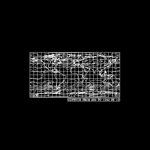
;----------- Begin first plot -----------------------------------------Draw a contour plot over a geographic map.
  resources@sfXCStartV = min(psl&lon)
  resources@sfXCEndV   = max(psl&lon)
  resources@sfYCStartV = min(psl&lat)
  resources@sfYCEndV   = max(psl&lat)
In order to overlay any plot on a map plot, you must specify the latitude and longitude values of where you want the plot to be overlaid on the map. This is done by specifying the X axis coordinates of the overlay plot in longitude coordinates, and the Y axis coordinates of the overlay plot in latitude coordinates.
For a contour plot, if your grid is equally spaced, then you can use the ScalarField resources sfXCStartV and sfXCEndV for setting the minimum and maximum values of the X axis, and sfYCStartV and sfYCEndV for setting the minimum and maximum values of the Y axis. If you have arrays of equally-spaced values representing your axes, then you can use the sfXArray and/or sfYArray resources instead, to set arrays of values.
If your grid is not equally spaced, then you must use the resources sfXArray and sfYArray as described in example 2 to define the whole range of values for both axes.
In this example, the *StartV and *EndV resources are being used to define the minimum and maximum latitude and longitude coordinates.
Since psl&lat and psl&lon are coordinate variables of psl, this means they represent the latitude and longitude values that psl is measured over. Thus, use these coordinate variables to provide the minimum and maximum latitude/longitude values for overlaying the contour plot. The functions min and max take arrays of any dimensionality and return the minimum and maximum values of that array.
Note: If you don't set any ScalarField resources for determining the minimum and maximum values of the X and Y axes, then the minimum values default to 0.0, and the maximum values default to n-1 and m-1 respectively, where n is the number of points of psl in the X direction, and m is the number of points of psl in the Y direction. This causes the contour plot to be overlaid at the latitude/longitude corners (0.,0.) and (m-1,n-1) which doesn't really make sense.
map = gsn_contour_map(wks,psl,resources)Create and draw a contour plot of the psl variable over a map. The default map projection is cylindrical equidistant. The first argument of the gsn_contour_map function is the workstation variable returned from the previous call to gsn_open_wks. The next argument is the 2-dimensional scalar field to be plotted and should be of type float, double, or integer. The last argument is a logical value indicating whether you have set any resources.
Note that the contour plot covers the full map. This is because the latitude values you specified in lines 31-34 go from -90 to 90, and the longitude values go from -180 to 180 (verify this by using print to print these values out).
It is important to note that the gsn_contour_map function is actually creating two plots, the contour plot and the map plot. The map plot is what's returned from the function, and the contour plot is returned as an attribute of the map plot called "contour." When you overlay one plot on another, the plot being overlaid is called the "base plot," and the plot that is overlaying the base plot is called the "overlay plot." The gsn_* functions that create such overlay plots always return the base plot as the function value, and the overlay plot as an attribute of the base plot. This information becomes useful when you use a statement called setvalues to change resources, as is done in example 9.
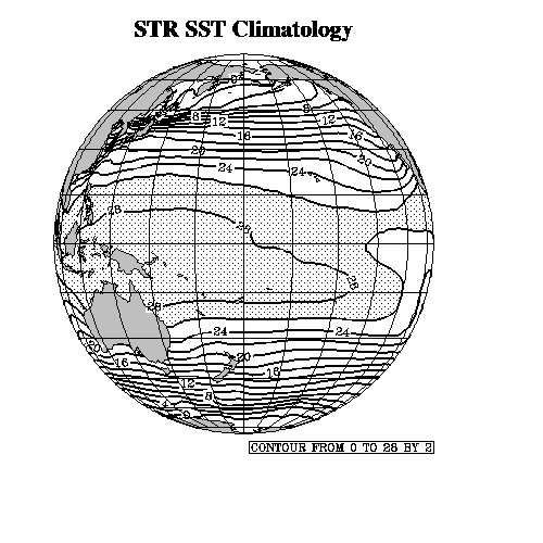
;----------- Begin second plot -----------------------------------------Draw a contour plot of the first time step of sst (sea surface temperature) over an orthographic projection, and set some resources to fill some of the contour levels with a stipple pattern, to mask the contours over land and to make the plot slightly larger. The concept of the drawing orders of contour and map components is introduced (for the purpose of getting the masking effect that you want).
  getvalues wks
    "wkColorMap" : cmap
  end getvalues
Use getvalues to retrieve the default
color map in use and store it to a local variable (cmap in
this case, but you can call this variable anything you want). The
color map is associated with the workstation that you opened in the
call to gsn_open_wks, so it is part of the group of "Workstation"
resources that start with "wk".The default color map has 32 entries (where each entry is an RGB value), so cmap is allocated by NCL as a 32 x 3 float array.
The getvalues statement is described in more detail in example 4.
  cmap(0,:) = (/1.,1.,1./)
  cmap(1,:) = (/0.,0.,0./)
  gsn_define_colormap(wks, cmap)
Color indices 0 and 1 represent the background and foreground colors respectively, and by default, the background color is black and the foreground color is white. Using the color map that you just retrieved (cmap), set the background to white and the foreground to black. Colors are set using RGB values, where white is represented by (1.,1.,1.) and black by (0.,0.,0.).
Details on creating your own color map are covered in example 2.
  resources@mpProjection = "Orthographic"
  resources@mpCenterLonF = 180.
Using the mpProjection resource, change the map projection to "Orthographic" (the default is "CylindricalEquidistant") and rotate the globe so that the center longitude is 180 (the default is 0). There are two kinds of map resources, one for map projections ("MapTransformation"), and one for all other map resources ("MapPlot"). Resources from both groups start with "mp".
There are ten different map projections to choose from, and they are documented in the resource description for mpProjection.
As noted in example 1, predefined strings are case-insensitive, so the mpProjection resource could have also been set using "orthographic" or "ORTHOGRAPHIC" or any another combination of uppercase and lowercase characters.
  resources@mpFillOn     = True
  resources@mpFillColors = (/0,-1,28,-1/)
Turn on the filling of geographical areas in the map with mpFillOn set to True. Each element of the mpFillColors array represents a specific geographic region to fill. Specify the colors for oceans, land, and inland water, respectively, by setting this array to various color index values (the first element is a special one that you don't need to worry about for now). The color index "-1" (also known as "transparent") is a special value indicating you don't want any fill, so in the array above, you are specifying that you don't want oceans and inland water to be filled, and you do want to fill land gray (color index 28 is gray in the default color map which is used here). There are actually six more elements of mpFillColors to set, but since you only want to fill land in this case, you don't need to worry about setting the rest of the elements of this array.
If you don't set mpFillColors, then default color index values are provided.
  resources@vpXF      = 0.1
  resources@vpYF      = 0.9
  resources@vpWidthF  = 0.7
  resources@vpHeightF = 0.7
Set some resources to change the size and location of the plot you want to draw in the viewport. The viewport is thought of as the canvas that you draw on, whose lower left corner is at (0.,0.) and upper right corner is at (1.,1.) (NDC coordinates). To position and resize a plot on a viewport, use NDC coordinates to specify the upper left corner of the plot and the height and/or width of the plot. The defaults of vpXF, vpYF, vpWidthF, and vpHeightF are 0.2, 0.8, 0.6, and 0.6 respectively.
Viewport resources are part of the "View" group and start with "vp".
  mnlvl = 0
  mxlvl = 28
  spcng = 2
  ncn   = (mxlvl-mnlvl)/spcng + 1

  resources@cnLevelSelectionMode = "ManualLevels"
  resources@cnMinLevelValF       = mnlvl
  resources@cnMaxLevelValF       = mxlvl
  resources@cnLevelSpacingF      = spcng
Set some resources to define your own contour levels. Setting the resource cnLevelSelectionMode to "ManualLevels" means that the resources cnLevelSpacingF, cnMinLevelValF, and cnMaxLevelValF are used to determine the contour levels. Contour levels are created starting with cnMinLevelValF, and spaced at intervals of the value of cnLevelSpacingF until cnMaxLevelValF is reached. The contour levels are stored in the array resource cnLevels, and in this case, are equal to (0,2,4,...,26,28).
The default of cnLevelSelectionMode is "AutomaticLevels", which means that the contour levels are chosen for you at "nice" values. The resource cnLevelSpacingF can be set by itself in this mode to determine the contour level spacing.
  resources@cnFillOn           = True
  resources@cnMonoFillColor    = True
  resources@cnMonoFillPattern  = False
  resources@cnFillPatterns     = new((/ncn+1/),integer)
  resources@cnFillPatterns(:)  = -1
  resources@cnFillPatterns(ncn-1:ncn) = 17
Set some resources for filling contour regions greater than 26 with a stipple fill pattern. Note that there is always one more fill area than there are contour levels. This is because all but the last index of cnFillPatterns specifies the fill pattern for any region containing a data value less than the corresponding value of cnLevels, while the last index of cnFillPatterns specifies the fill pattern for regions containing data values greater than the value of cnMaxLevelValF. Since cnLevels has the values (0,2,4,...,28), this means index 0 of cnFillPatterns is for all regions containing values less than 0, index 1 is for region values greater than 0, but less than 2, etc. Index 14 of cnFillPatterns is for region values greater than 26, but less than 28, and index 15 is for region values greater than 28.
To stipple all regions whose values are greater than 26, set the last two elements of cnFillPatterns to 17 (ncn is the number of contour levels, which was calculated in line 62). The rest of the contour levels are set to transparent (index -1).
  resources@cnLineDrawOrder      = "Predraw"
  resources@cnFillDrawOrder      = "Predraw"
In order to understand how overlaying a plot on a map works, you need to understand something about the drawing order of the various components of the two plots (the map plot and the overlay plot). Also, by being able to specify different drawing orders for the various components of both plots, you can get different masking effects.
[Take a deep breath.]
There are three drawing orders available: "Predraw", "Draw", and "Postdraw". Components drawn during the "Predraw" phase are drawn before components drawn in the "Draw" phase, which, in turn, are drawn before components in the "PostDraw" phase.
The contour plot has three components for which you can specify a drawing order: contour lines, contour filled areas, and contour line labels. The map plot has five components: map outlines, map labels, latitude/longitude grid lines, map fill, and a perimeter.
By default, when a contour plot is drawn over a map plot, all of the contour plot components, the map filled areas, and the map perimeter are drawn during the "Draw" phase, and the map outlines, grid lines, and map labels are drawn during the "Postdraw" phase. Note that only the components that are drawn by default or explicitly set by you are drawn (for example, map filled areas are not drawn by default).
If you set both mpFillOn and cnFillOn to True (as you have done in this case), then you also have to manage the drawing order of the contour and map filled areas, otherwise one will completely cover the other (since they are both drawn during the "Draw" phase). For example, let's assume you want to fill the land areas with a color, and draw filled contours with contour lines over the ocean only. In this case, you want to draw the contour components before you draw the filled land areas, so the land areas effectively mask the contour filled areas. This is accomplished by setting the contour draw order resources cnLineDrawOrder and cnFillDrawOrder to "Predraw" to force these components to be drawn before the filled map areas.
Note that cnLabelDrawOrder is not being set to anything. This is because the contour line labels just happen fall over the oceans areas mostly, and thus it is not necessary to specify that they get drawn in the "Predraw" phase.
  resources@sfXCStartV = min(sst&lon)
  resources@sfXCEndV   = max(sst&lon)
  resources@sfYCStartV = min(sst&lat)
  resources@sfYCEndV   = max(sst&lat)
Set these four ScalarField resources to indicate the latitude and longitude values for overlaying the contour plot on the map.
map = gsn_contour_map(wks,sst(0,:,:),resources)Create and draw a contour plot of the first time step of the sst variable over an orthographic map projection. If you watch the frame as it is being drawn, you will see the contour lines and areas being drawn first, then the filled land areas, and then the contour line labels.
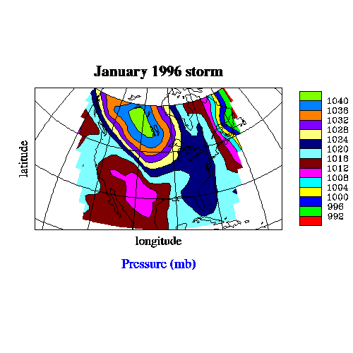
;----------- Begin third plot -----------------------------------------Draw a contour plot of the first time step of the pf (pressure) variable over a Lambert equal area projection, and set some resources to fill all of the contour levels and to limit the area of the map view.
  delete(resources)
  resources = True
Start with a new list of resources.
  resources@sfXCStartV = min(pf&lon)
  resources@sfXCEndV   = max(pf&lon)
  resources@sfYCStartV = min(pf&lat)
  resources@sfYCEndV   = max(pf&lat)
Set these four ScalarField resources to indicate the latitude and longitude values for overlaying the contour plot on the map.
  resources@mpProjection = "LambertEqualArea"
  resources@mpCenterLonF = (pf&lon(pf@nlon-1) + pf&lon(0))/2
  resources@mpCenterLatF = (pf&lat(pf@nlat-1) + pf&lat(0))/2
Change the map projection to "LambertEqualArea" and change the center longitude and latitude values to be the center of the latitude/longitude ranges defined by pf's coordinate variables, lat and lon.
  resources@mpLimitMode = "LatLon"
  resources@mpMinLonF   = min(pf&lon)
  resources@mpMaxLonF   = max(pf&lon)
  resources@mpMinLatF   = min(pf&lat)
  resources@mpMaxLatF   = max(pf&lat)
Since the pf data does not cover the whole map, zoom in on the part of the map that does contain the data. Verify what latitude/longitude area the pf data is measured over by adding the following four lines to the NCL script:
  print(min(pf&lat))
  print(max(pf&lat))
  print(min(pf&lon))
  print(max(pf&lon))
These print values indicate that the longitude values range from -140 to -52.5, and that the latitude values range from 20 to 60, which is the area surrounding the United States.
When mpLimitMode is set to "LatLon", the resources mpMinLonF, mpMaxLonF, mpMinLatF, and mpMaxLatF are used to determine the limits of the maximum viewable portion of the map in latitude/longitude coordinates. When you zoom in on a map in this manner, the zoomed portion of the map is enlarged to fit the viewport specified.
  resources@vpXF      = 0.1
  resources@vpYF      = 0.9
  resources@vpWidthF  = 0.7
  resources@vpHeightF = 0.7
Change the size and location of the plot within the viewport.
  resources@gsnScale = True
  resources@gsnFrame = False
The resources gsnScale and gsnFrame are special ones recognized only by the gsn_* suite of plotting functions.
In NCL, if the viewport of a plot is something other than a square, then the X and Y axis labels are scaled proportionally. For example, if the Y axis is half the length of the X axis, then the Y axis label will be approximately half the size of the X axis label. To work around this, set gsnScale to True. This tells the plotting function in question that you have changed the aspect ratio of the plot to a non-square, but that the the X and Y axes labels should stay the same size. The new size of these labels will be an average of the two original sizes.
Also by default, the frame of the workstation is automatically advanced unless you set gsnFrame to False. If you want to annotate the plot with text strings after you draw it, then you don't want to advance the frame just yet.
map = gsn_contour_map(wks,pf(0,:,:)*0.01,resources)Create and draw a filled contour plot of the first time step of the pf variable over a Lambert equal area map projection. Note that the pressure values are being converted from Pascals to millibars in this call, by multiplying all the pf values with 0.01.
  txres               = True
  txres@txFontHeightF = 0.025
  txres@txFontColor   = 4
  gsn_text_ndc(wks,":F25:Pressure (mb)",.45,.25,txres)
The procedure gsn_text_ndc allows you to draw text anywhere within the viewport. The first argument of gsn_text_ndc is the workstation variable returned from the previous call to gsn_open_wks and the second argument is the string to draw. The next two arguments are the X and Y locations of the text in NDC coordinates, and the last argument is a logical value indicating whether you have set any resources. The text string is centered around the X and Y locations that you specify, unless you set some resources to do otherwise.
Text resources are part of the "TextItem" group and start with the letters "tx". You are using resources here to change the default font height and color of the text string (the default values are 0.05 and 1, respectively). The ":F25:" part of the string is a text function code which changes the font to "Times-Roman." Text function codes are discussed in example 3.
It is important not to confuse TextItem resources with Title resources described in previous examples. Title resources are specifically for controlling the look of the main title at the top of the plot, and the labels for the X and Y axes. TextItem resources are for generic text to be placed anywhere within the viewport.
Line 138:
frame(wks)
Since you set gsnFrame to False, you need to advance
the frame by calling frame. The variable
wks is the one returned from a previous call to
gsn_open_wks.
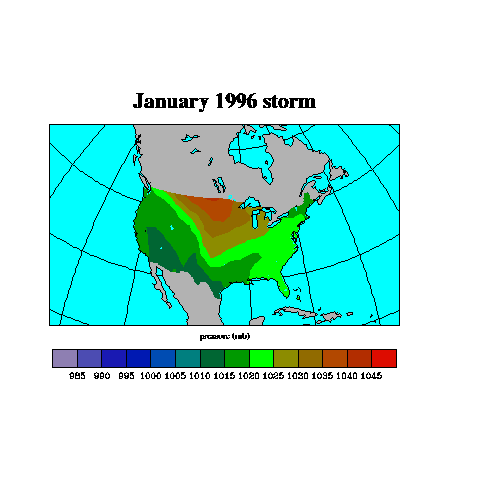
;---------- Begin fourth plot ------------------------------------------Draw a contour plot of the second time step of the pf variable over a Lambert equal area projection, and set some resources to fill the contour levels, to limit the area of the map view, and to mask the contours over everything but the United States.
  delete(resources@tiXAxisString)
  delete(resources@tiYAxisString)
  delete(resources@gsnFrame)
If don't want a resource that you set earlier to apply to a new plot, remove it with delete.
  delete(cmap)
  cmap = (/(/1.00, 1.00, 1.00/), (/0.00, 0.00, 0.00/), \
           (/.560, .500, .700/), (/.300, .300, .700/), \
           (/.100, .100, .700/), (/.000, .100, .700/), \
           (/.000, .300, .700/), (/.000, .500, .500/), \
           (/.000, .400, .200/), (/.000, .600, .000/), \
           (/.000, 1.00, 0.00/), (/.550, .550, .000/), \
           (/.570, .420, .000/), (/.700, .285, .000/), \
           (/.700, .180, .000/), (/.870, .050, .000/), \
           (/1.00, .000, .000/), (/0.00, 1.00, 1.00/), \
           (/.700, .700, .700/)/)

  gsn_define_colormap(wks, cmap)
Define a new color map. Since you used the variable cmap
earlier to retrieve the default color map, you need to delete it first
because the new color map you are creating is a different size. In
NCL, once you create a variable, it cannot change size unless you
delete it first and recreate it.
  resources@mpFillOn              = True
  resources@mpFillAreaSpecifiers  = (/"water","land","USStatesWater"/)
  resources@mpSpecifiedFillColors = (/17,18,17/)
  resources@mpAreaMaskingOn       = True
  resources@mpMaskAreaSpecifiers  = "USStatesLand"
To draw contours over the United States only and fill the rest of the map areas with a color, you need to set some resources to do the filling and masking. You need to set map fill (mpFillOn) and masking (mpAreaMaskingOn) to True, and you also need to specify which areas to fill (mpFillAreaSpecifiers) and which areas to mask (mpMaskAreaSpecifiers). The areas "Water", "Land", "USStatesLand", etc., are from a set of predefined string constants that define map areas by category. The way area masking works is that you first specify what areas to fill, and then you specify what areas to "subtract" or mask. In this case, you are specifying that you want to fill all the map areas except for the United States land areas (the Great Lakes will be filled).
resources@mpGridMaskMode = "MaskLand"Draw the map grid lines over everything but land. There are other pre-defined strings available for mpGridMaskMode, and they are specified in the documentation for that resource. The default is "MaskNone" which means to draw the grid lines over the whole map.
resources@cnFillDrawOrder = "Predraw"The way area masking works for maps is that a "hole" is left in the areas of the map that you specified with the mpMaskAreaSpecifiers resource, so if you draw the filled contours first and then the map, the filled contours are visible through this "hole."
  resources@cnLevelSelectionMode = "ExplicitLevels"
  resources@cnLevels             = fspan(985.,1045.,13)
Set cnLevelSelectionMode to "ExplicitLevels" to indicate that you want to define your own contour levels with the cnLevels resource. The fspan function returns an array of evenly spaced floating point numbers. The first argument is the starting value, the second argument is the ending value, and the third argument is the number of points to create. In this case, fspan returns an array of 13 elements equal to (985.,990.,995.,...,1040.,1045.).
  resources@pmLabelBarSide = "Bottom"
  resources@lbOrientation  = "Horizontal"
Since the PlotManager "manages" the label bar that's associated with the contour plot (the one that you turned on by setting pmLabelBarDisplayMode to True in the third frame of this example), you need to use a PlotManager resource to move the label bar to another location. In this case, you use pmLabelBarSide to move it to the bottom of the plot (the default is to the right), and then you use the LabelBar resource lbOrientation to make it horizontal.
map = gsn_contour_map(wks,pf(1,:,:)*0.01,resources)Create and draw a filled contour plot of the second time step of the pf variable over a Lambert equal area map projection. Also, convert pf from Pascals to millibars in the same step.