Basics
This chapter contains information that is essential to a sound understanding of NCL at a beginning level; it is meant to augment and complement the content in the "Learning NCL by example" chapter. After studying the examples and reading this chapter, you will be prepared to read the chapter on "Going Beyond the Basics," which will give you a more thorough understanding of NCL.
Variables
NCL variables are more general than variables used by traditional programming languages such as Fortran and C. Variable names are case sensitive ("Square" is different from "square"), and in addition to having assigned values, NCL variables may have associated ancillary information called metadata. There are three types of metadata:attributes
An attribute of a variable is information about the variable. Examples of such information are: a minimum value for the variable, a maximum value for the variable, and descriptive information about the variable (for example, its units). Attributes of a variable are created and referenced using the "@" symbol. An attribute is created by referencing it on the left side of an assignment statement. Attributes can be created only for existing NCL variables.For example, if x is an NCL variable, then the lines:
x@min = -50
x@max =  50.d
x@units = "meters"
x@long_name = "A variable for temporary storage"
x@eigenvalues = (/ 0.75, 0.40, 0.01 /)
would create the attributes min, max, units, long_name, and eigenvalues. In the above, notice that NCL arrays are initialized by bracketing the data with the array designator characters "(/" and "/)".
Attributes have types, so, using the attributes created above, the lines:
xmini = x@min
xmaxr = x@max
info = x@long_name
eigval = x@eigenvalues
would create an NCL variable xmini of type integer, an NCL variable xmaxr of type double (a 'd' after a value automatically makes that value a double), an NCL variable info of type string, and a singly-dimensioned float array eigval.
The attribute "_FillValue" is special in NCL and, if defined, denotes the value that, when stored in a variable, will be considered as a missing value. An array may have several occurrences of the missing value in it. These missing values are subsequently ignored by the plotting functions and by many of the computational functions.
The NCL function isatt can be used to query whether a given string is an attribute name for a variable.
named dimensions
Integer dimensions define the shape (number of dimensions) and size (number of elements for each dimension) of a variable. A singly-dimensioned variable of size one is called a scalar variable (or simply a scalar). By convention, dimensions are numbered from 0 to n-1 where n is the number of dimensions (the shape) of the data referenced, and the leftmost dimension is numbered 0.An array dimension can be assigned a name. This can be done by entering an array name followed by the "!" character followed by an integer dimension number and setting that equal to a name (string value). For example, if the variable pressure has three dimensions, then the statements:
pressure!0 = "time"
pressure!1 = "latitude"
pressure!2 = "longitude"
would assign the name "time" to the first dimension of pressure, "latitude" to the second dimension, and "longitude" to the third. These dimension names can be used in "named subscripting," discussed in the "Array subscripting" section below. Named dimensions are also used to define coordinate variables as discussed immediately below.
The NCL function isdim can be used to query if a given string is the name of a named dimension of a variable.
coordinate variables
NCL allows for indexing arrays with user-defined coordinate subscripts. To see why this is desirable, consider the case where temperature is a 2-dimensional NCL variable defined on the globe at 5-degree intervals in longitude and latitude. If you want to access the value of temperature at 35 degrees latitude and 70 degrees longitude, it would be more intuitive to use those coordinate values as indices, rather than figure out what the standard subscript values are for that coordinate.You can define a coordinate variable for any named dimension of an array, and only for a named dimension. Suppose, for example, that pressure is a 9x7 array and consider the statements:
pressure!0 = "lat"
pressure!1 = "lon"
lat_points = (/-80, -60, -40, -20, 0, 20, 40, 60, 80/)
lon_points = (/-180, -120, -60, 0, 60, 120, 180/)
pressure&lat = lat_points
pressure&lon = lon_points
The first two statements name the first two dimensions of pressure, the next two statements define coordinate arrays, and the final two statements define the coordinate variables lat and lon and associate them with the coordinate arrays lat_points and lon_points respectively.
The coordinate array associated with a coordinate variable must have the same size as the named dimension with which the coordinate variable is associated. Also, a coordinate variable must have the same name as its corresponding named dimension. The elements in a coordinate array must be monotonically increasing or decreasing. Any of the numeric data types may be used for values in the coordinate arrays associated with a coordinate variable.
The use of coordinate variables for subscripting of arrays is described below in the "Array subscripting" section.
The NCL function iscoord can be used to query if a specified string is a coordinate variable of a variable.
Array subscripting
Much of NCL's usefulness for data processing derives from its strong array processing capabilities. These are similar to those of Fortran 90. The arithmetic operators apply to arrays as well as scalars so that arrays can be efficiently added, multiplied, compared, and so forth. NCL also automatically handles missing values.NCL's array subscripting syntax contributes significantly to NCL's data processing power and versatility. There are three types of subscripting:
standard subscripting
This is similar to the array subscripting in Fortran 90. For NCL standard array subscripts, the leftmost dimension is numbered "0" and the other dimensions are numbered in sequence, left-to-right. The dimension numbered "0" is referred to as the first dimension of the array, the dimension numbered "1" as the second dimension, and so forth. The leftmost dimension is the slowest varying, and the rightmost dimension is the fastest varying (i.e., arrays are stored in the "row x column" format familiar to C programmers). The subscripts used in standard subscripting are integers.The most general form of a standard subscript is m:n:i which indicates the range m to n in strides of i.
Consider the array v defined by
v = (/0,1,2,3,4,5,6,7,8,9/)then the following NCL statements illustrate the many possibilities for standard subscripts (semi-colons on an NCL statement initiate comments that are ignored by the NCL interpreter):
v1 = v(1:7)    ; v1  contains 1,2,3,4,5,6,7 .

v2 = v(1:7:3)  ; v2  is an array containing the
               ;       elements 1,4,7 .

v3 = v(:4)     ; v3  contains 0,1,2,3,4 (a missing
               ;       initial integer indicates
               ;       the beginning of the indices).

v4 = v(8:)     ; v4  contains 8,9 (a missing second
               ;       index indicates the largest
               ;       of the indices).

v5 = v(:)      ; v5  equals v (this is the same as
               ;       setting v5 = v).

v6 = v(2:4:-1) ; v6  contains 4,3,2 (in that order).
               ;       The algorithm is to find all
               ;       numbers within the range of
               ;       the first colon-separated
               ;       pair, then step in reverse
               ;       when the stride is negative.

v7 = v(6)      ; v7  is a scalar with value 6 .

v8 = v(5:3)    ; v8  contains 5,4,3 in that order
               ;       (when the starting index is
               ;       greater than the ending index,
               ;       a reverse selection is done).

v9 = v(::-1)   ; v9  contains 9,8,...,0 in that order.
The 1-dimensional case carries over to arrays with multiple dimensions, so that if w were a 5x7x11 array, the statement
w1 = w(0:4:2, :3, :)would define w1 as a 3x4x11 array constructed in each dimension as in the linear array example above.
named subscripting
Named subscripting allows you to reorder arrays. Named subscripting is allowed only if all dimensions of an array are named dimensions. If the variable pressure has two dimensions with the first dimension (dimension number 0) being named lat with size 19 and with the second dimension (dimension number 1) being named lon with size 37, then the statementpressure_rev = pressure (lon | :, lat | 4:5)would define pressure_rev as an array with first dimension named lon of size 37 and second dimension named lat of size 2. The syntax requires the vertical bars be present as well as a specified subscript range.
coordinate subscripting
Coordinate subscripting uses coordinate variables (as discussed above). Curly braces "{" and "}" are used to distinguish coordinate subscripts from standard subscripts. Otherwise all of the rules for standard subscripts apply.For example, where
w        = (/0,1,2,3,4,5,6/)              ; create data array
w!0      = "w_dim0"                       ; name the dimension
w&w_dim0 = (/.0, .1, .2, .3, .4, .5, .6/) ; associate array
ws       = w( {.1 : .5 : 2} )             ; use coord. subscripting
ws would be a 1-dimensional integer array of size 3 with
values 1,3,5. Note that the stride must always be an integer and should
be thought of as a skip indicator rather than an additive increment
value, since coordinate subscripts may not always be integers, as
illustrated here. A stride of 2 means to take every second value
after the first, a stride of 3 means take every third value, and so
forth.
Color maps
Color maps, also known as color tables, are generally represented by n x 3 arrays of red, green, and blue float values (referred to as RGB values) ranging from 0.0 to 1.0 (to indicate the intensity of that particular color). The first entry in a color map is the background color, and the second entry is the foreground color.NCL provides a default color map that contains 32 different colors, including a black background and a white foreground. If you want to define your own color map, then you can do it one of several ways:
- by using one of several predefined color maps (the default being one of them),
- by defining a set of RGB values,
- by defining a combination of named colors and RGB values, or
- by using HSV values.
Using a predefined color map
NCL provides several predefined color maps that range from 8 color entries to 255 color entries. It uses the one called "default" if you don't create your own color map. To use one of the predefined color maps, select one from the "Color table gallery", and set the resource wkColorMap to this name.For example, if you want to use the "temp1" color map, you can make this color map active by including the following setvalues statement:
setvalues wks
  "wkColorMap" : "temp1"
end setvalues
or the following GSUN statement:
gsn_define_colormap(wks,"temp1")after a workstation is opened (either from a call to gsn_open_wks or by using create to create a workstation).
Creating your own color map using RGB values
To create your own color map using RGB values, define a 2-dimensional float array dimensioned n x 3, where the first dimension represents the number of colors (n), and the second dimension represents the RGB values. Then, make it active by passing the variable containing the color map array to gsn_define_colormap, or by using the variable in a setvalues call. For example, if you open a workstation and create a color map array with the following NCL code:
  wks = gsn_open_wks("x11","example")

  cmap = (/(/1.00, 1.00, 1.00/), (/0.00, 0.00, 0.00/), \
           (/.560, .500, .700/), (/.300, .300, .700/), \
           (/.100, .100, .700/), (/.000, .100, .700/), \
           (/.000, .300, .700/), (/.000, .500, .500/), \
           (/.000, .700, .100/), (/.060, .680, .000/), \
           (/.550, .550, .000/), (/.570, .420, .000/), \
           (/.700, .285, .000/), (/.700, .180, .000/), \
           (/.870, .050, .000/), (/1.00, .000, .000/)/)
then you can make this new color map active with either of these segments of code:
gsn_define_colormap(wks,cmap)or
  setvalues wks
    wkColorMap" : cmap
  end setvalues
To help determine what RGB values to use to get the colors you want,
below are five color tables with sample RGB values. Each table has a
fixed intensity value for red, and shows the colors for varying
intensity values of blue and green:
| Table 1 | Table 2 | Table 3 | Table 4 | Table 5 |
|---|---|---|---|---|
| 
| 
| 
| 
|
| (Click on any table to see it enlarged.) | ||||
Note: To create a grayscale color map, use RGB values that are equal in intensity. For example, (0.11, 0.11, 0.11), (0.5, 0.5, 0.5), and (0.968, 0.968, 0.968) are all RGB values that produce varying shades of gray.
Creating your own color map using named colors and/or RGB values
To create a color map using a combination of color names and RGB values (as described above), create a 1-dimensional string array where each entry is either a color name or an RGB value (enclosed in double quotes). The 650 valid named colors are listed in the last column of the file "$NCARG_ROOT/lib/ncarg/database/rgb.txt." You can also see the color names and their associated colors by clicking on any one of the 15 tables below:
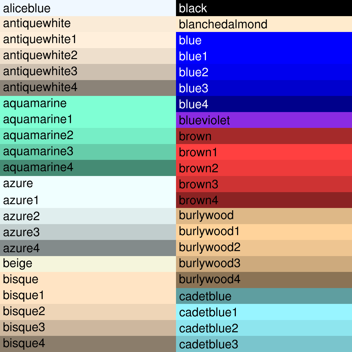
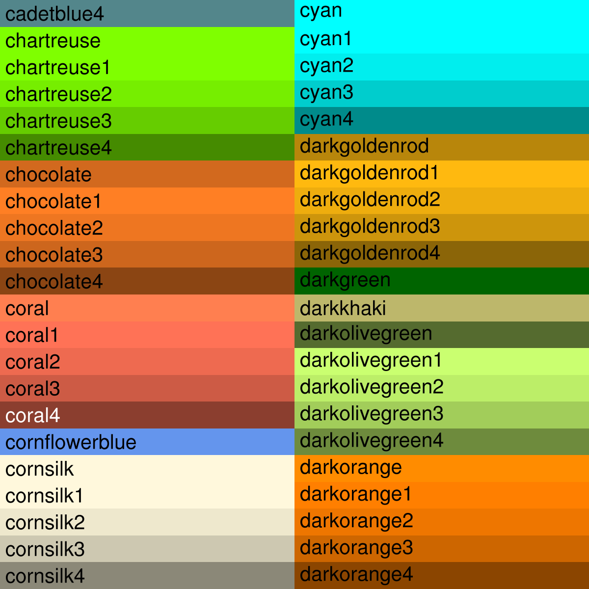
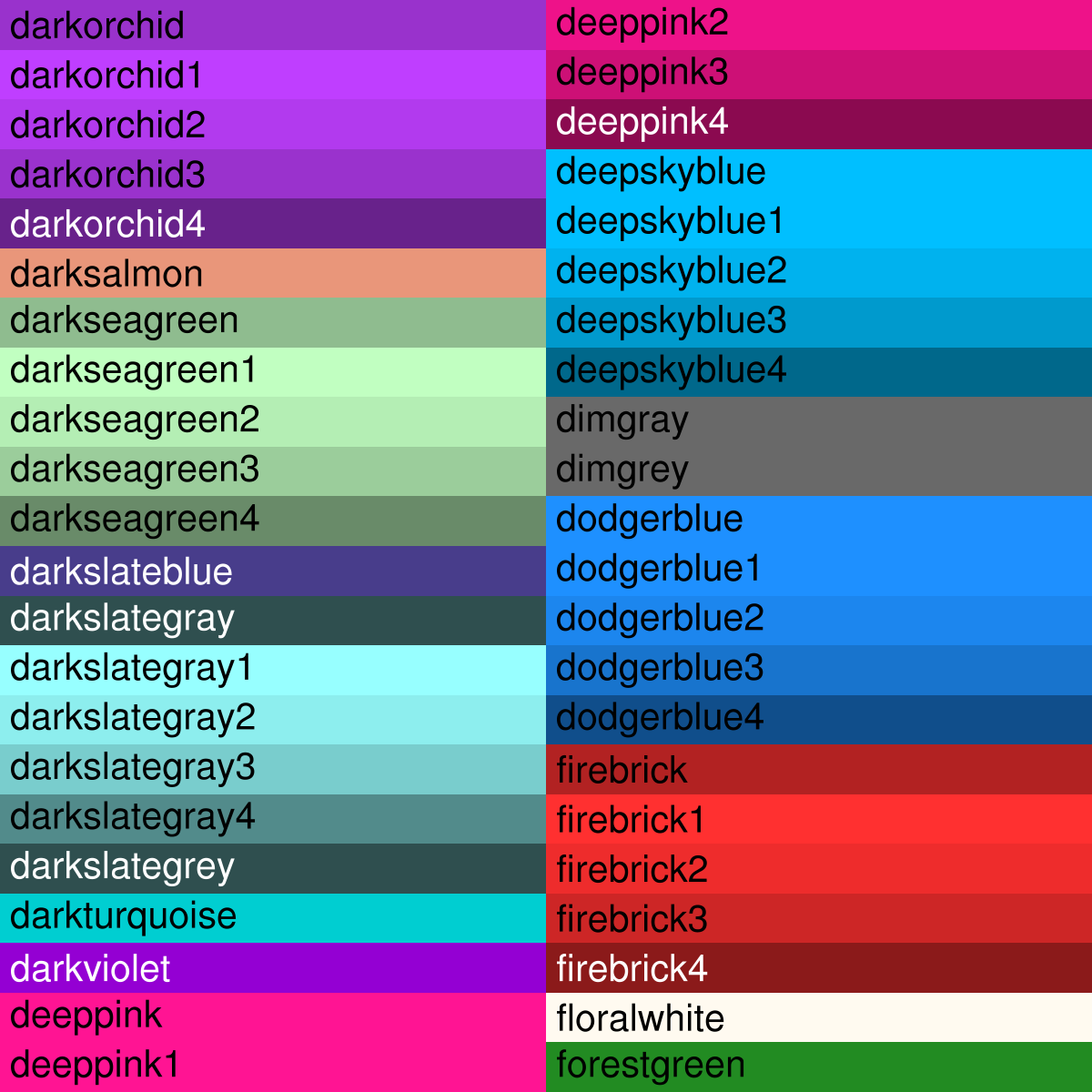
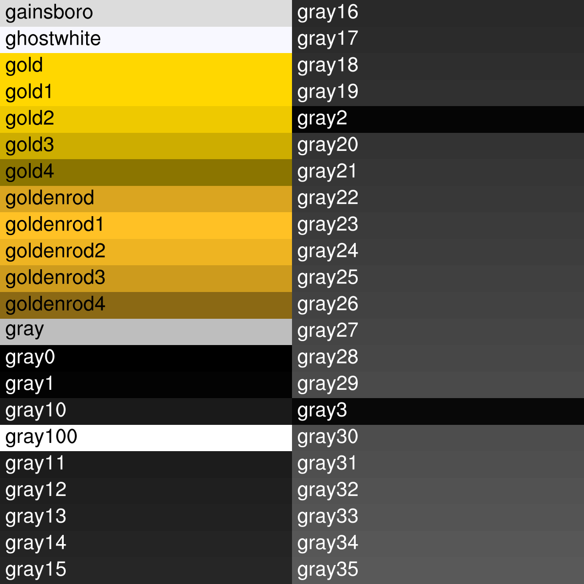
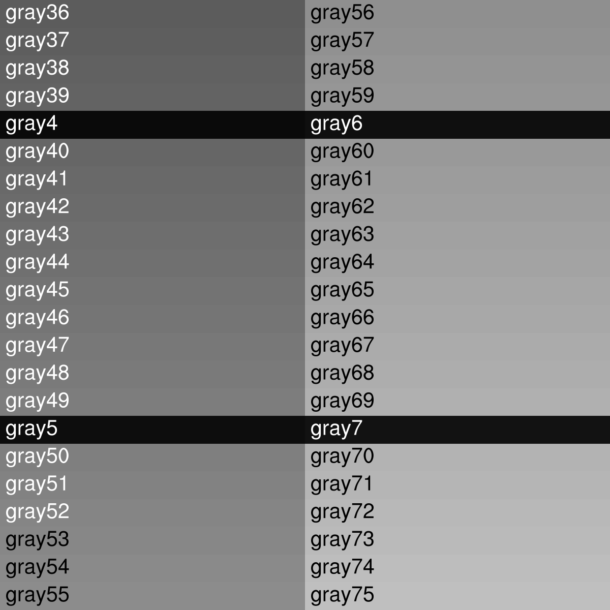
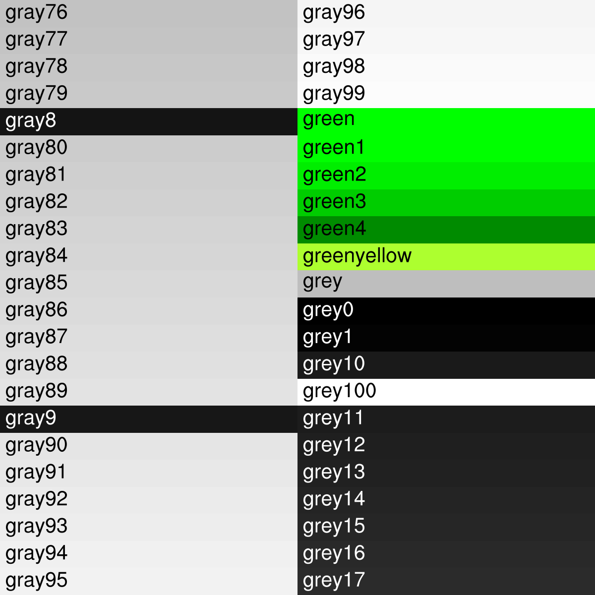
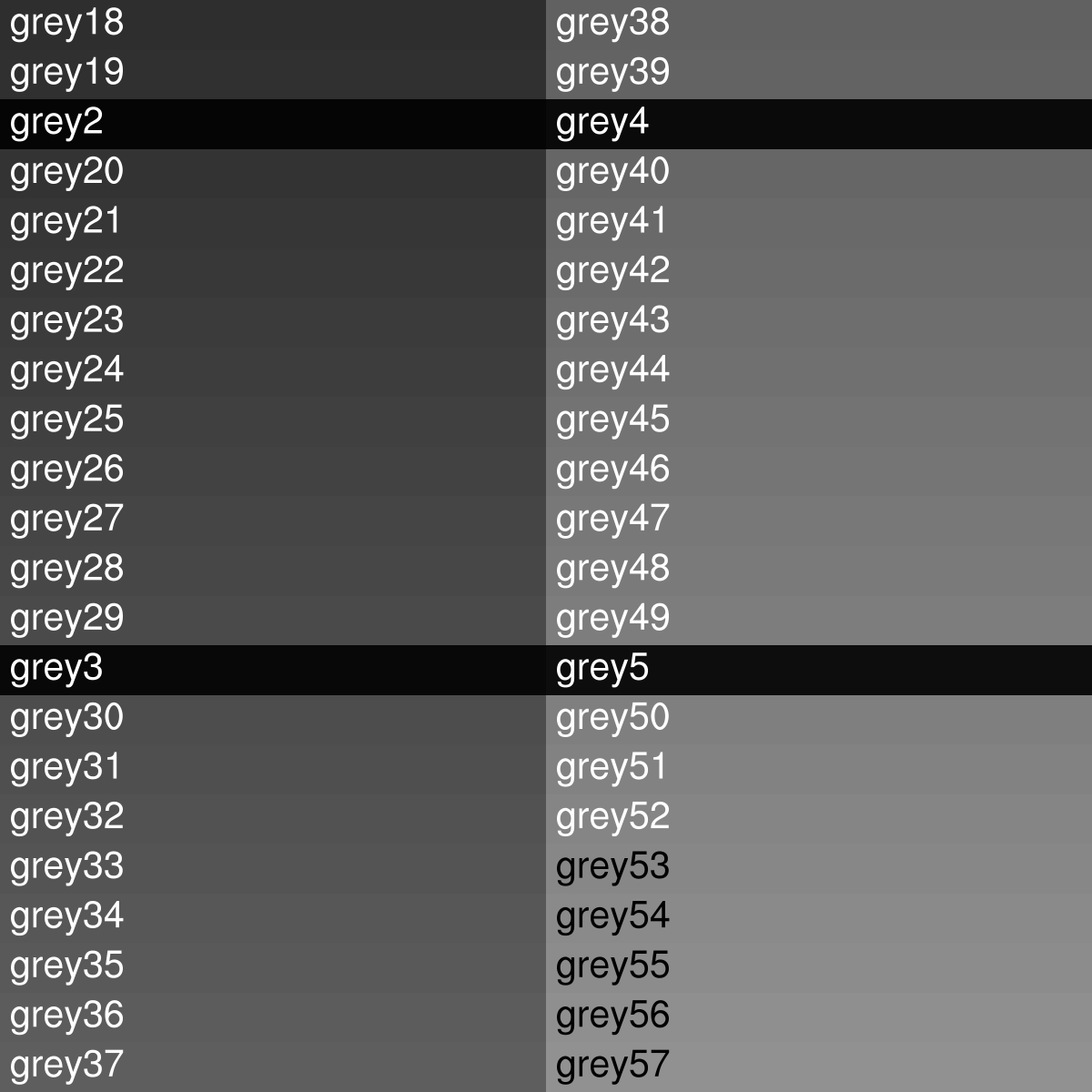
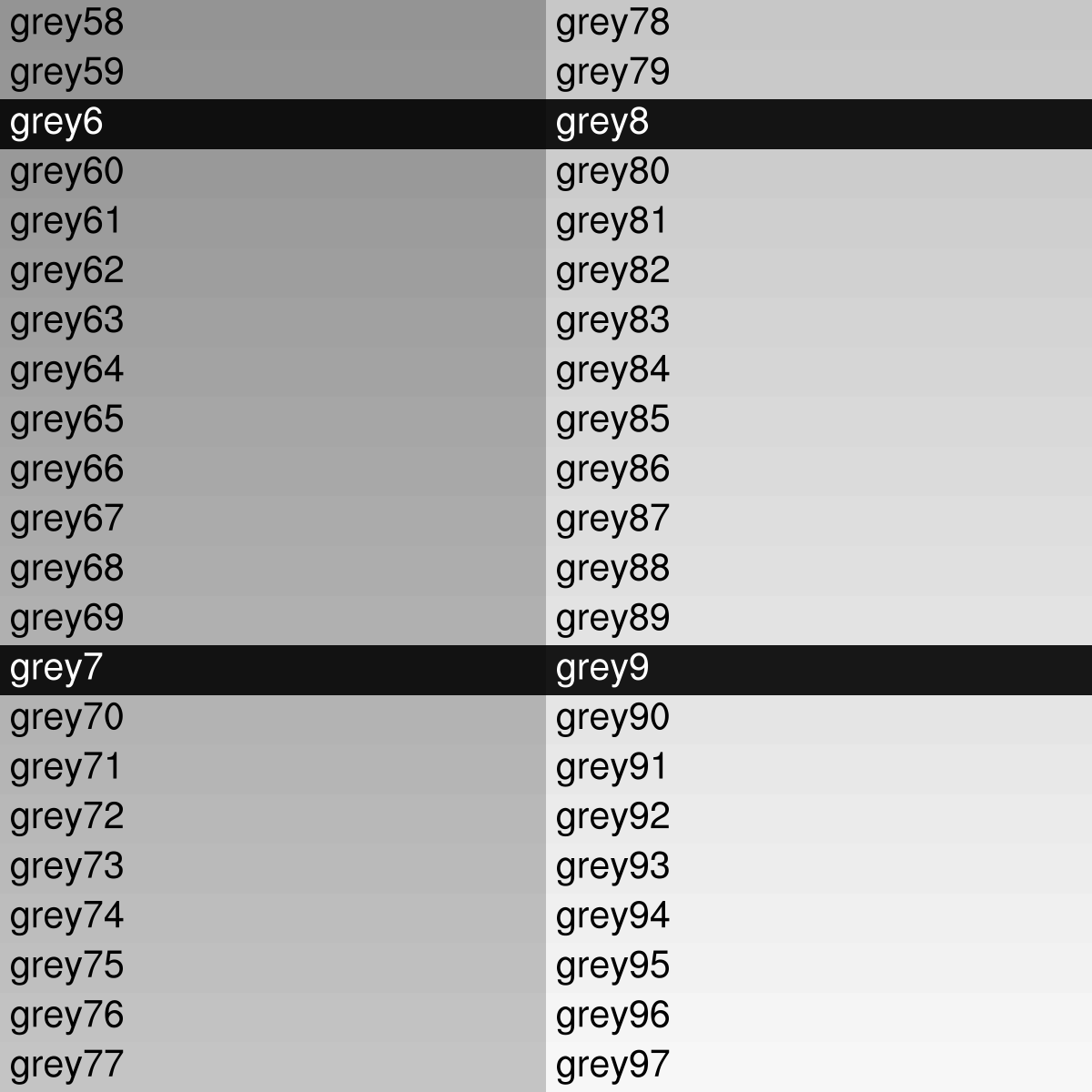
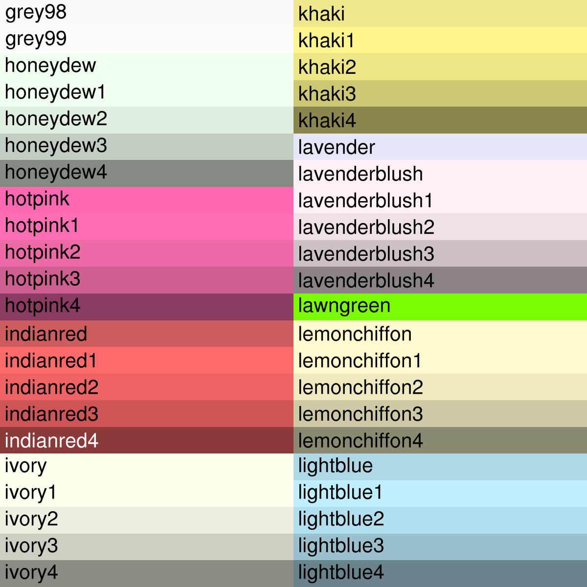
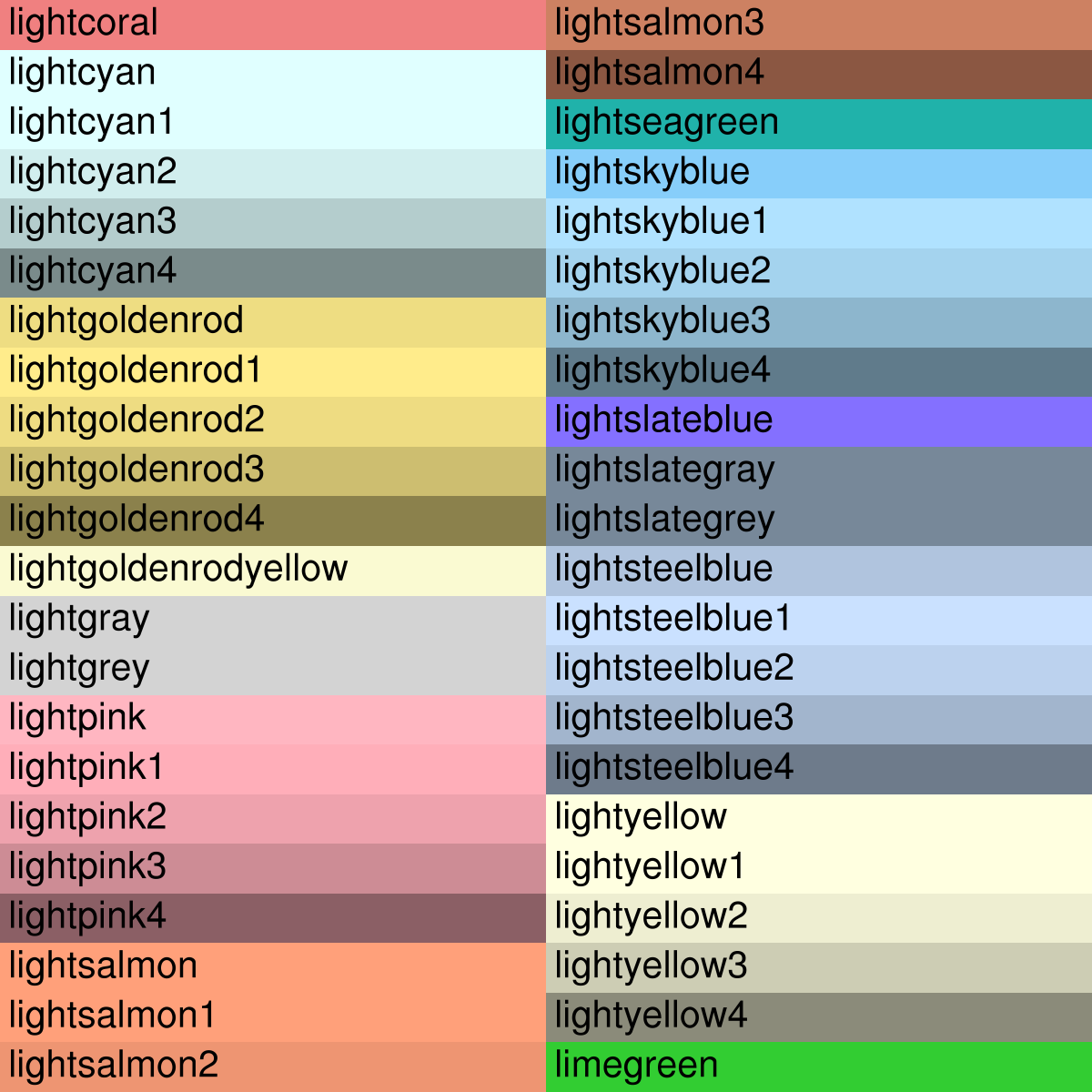
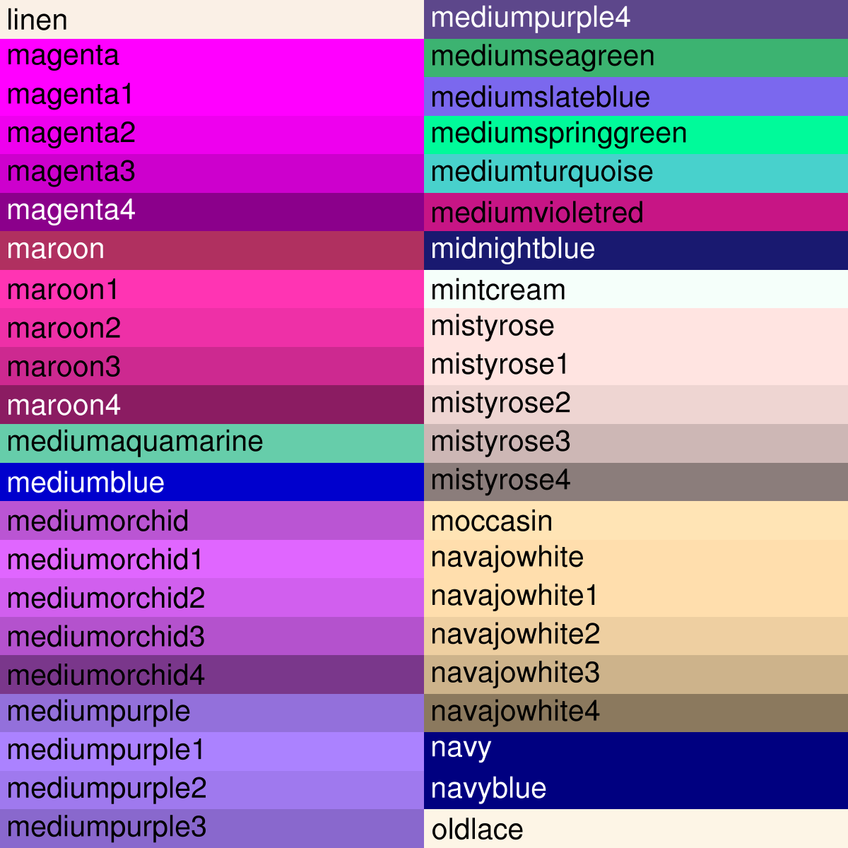
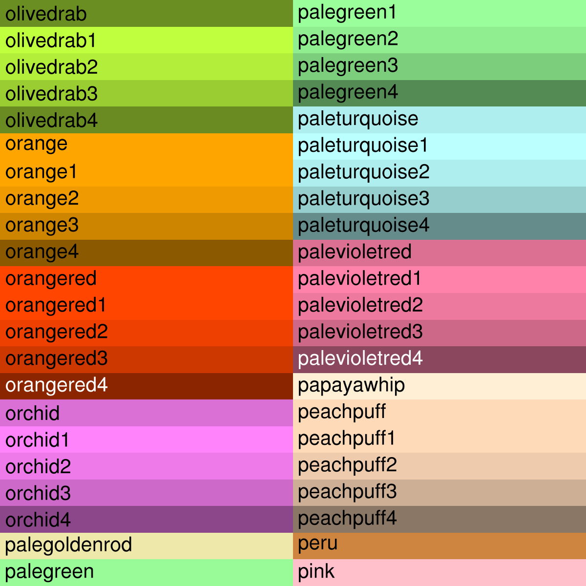
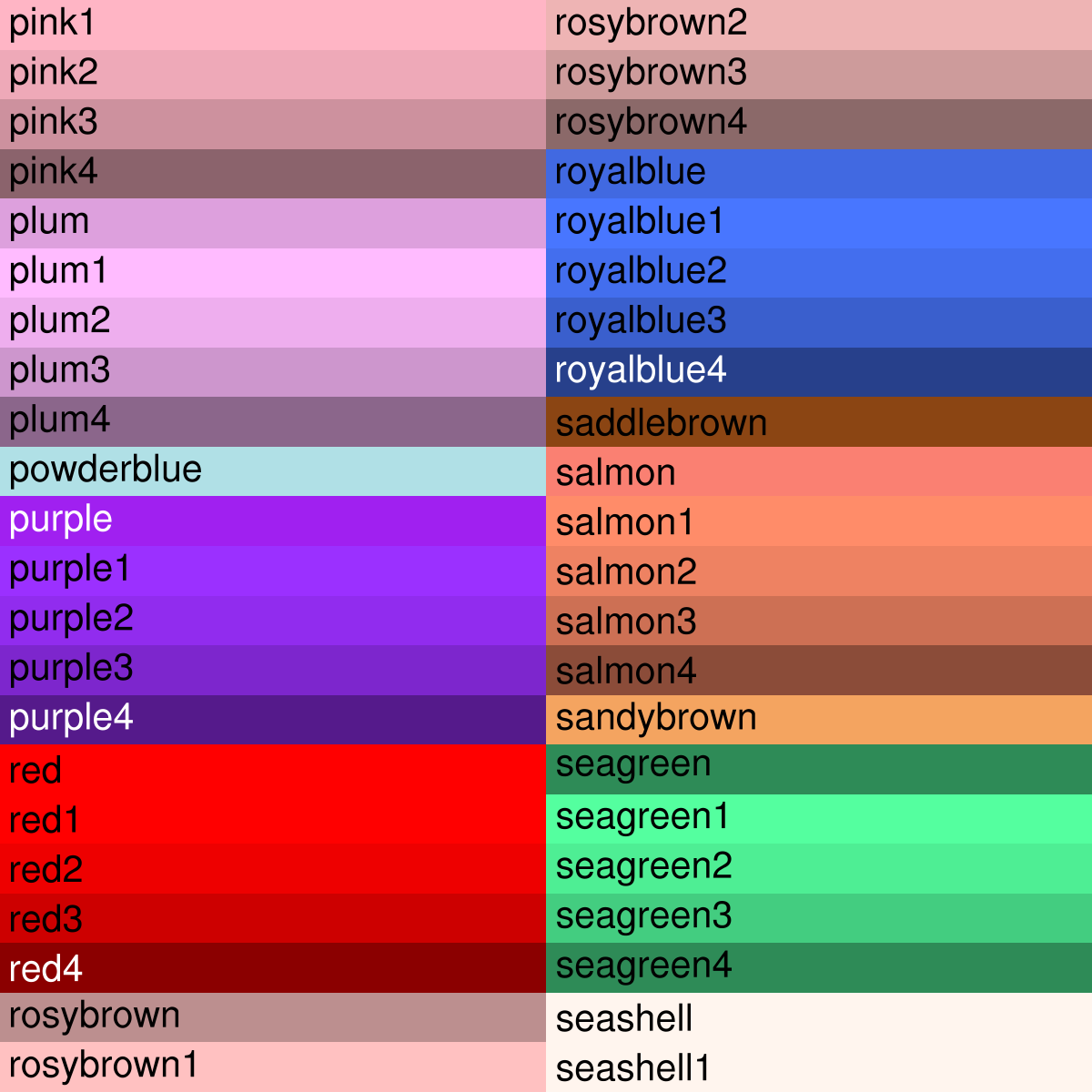
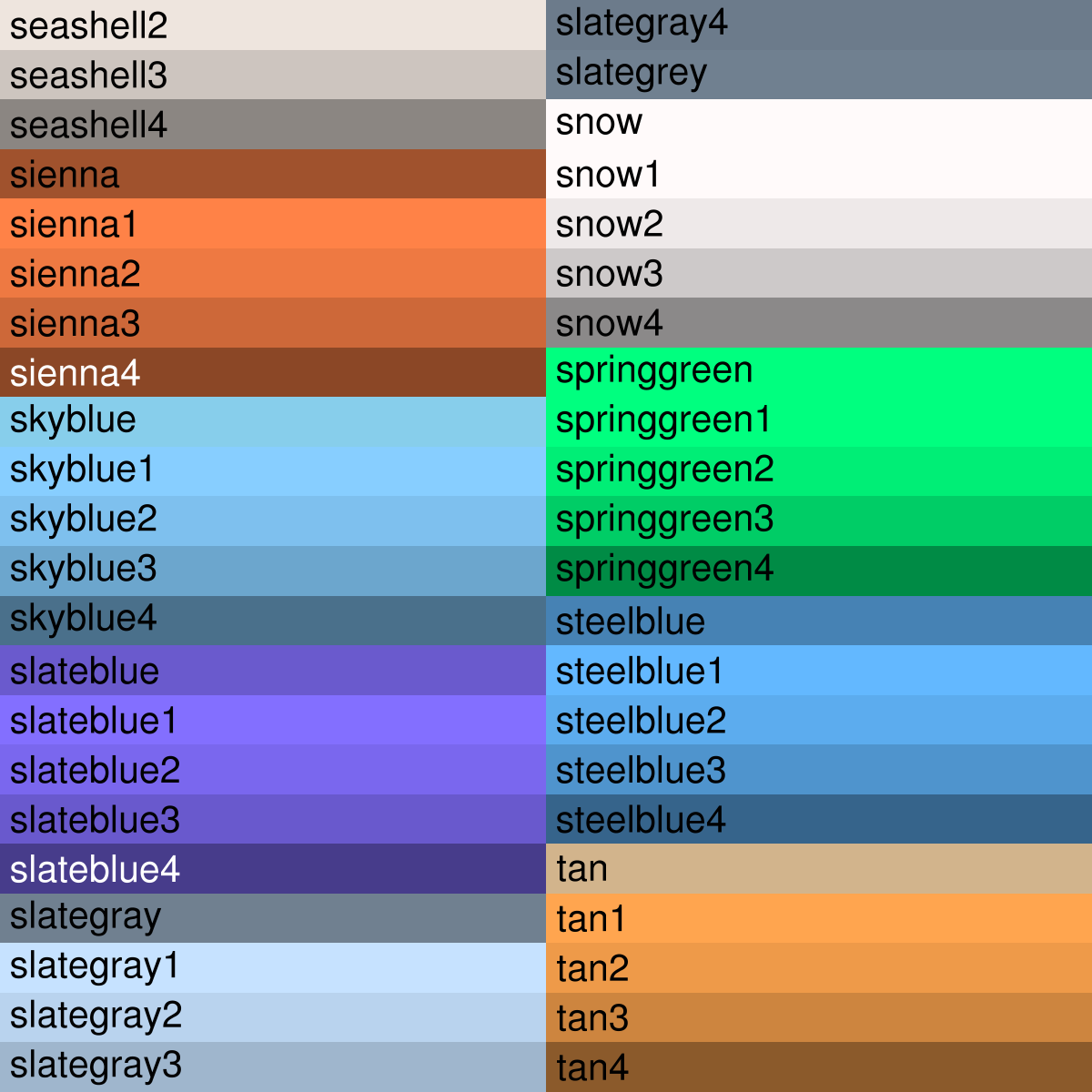
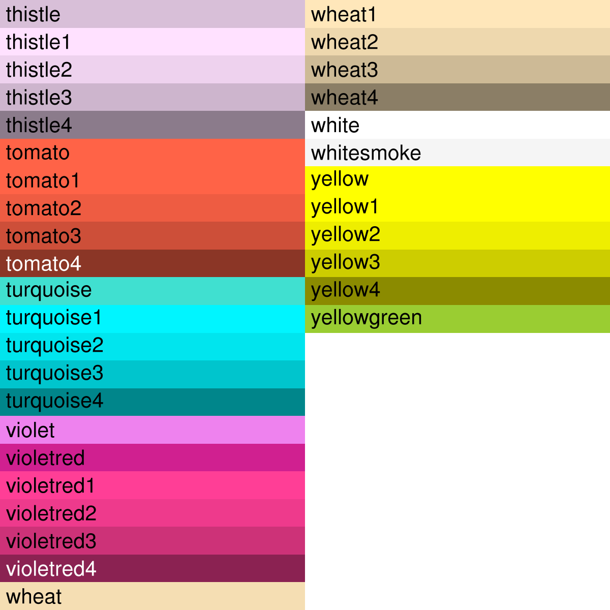
(Note that some of the colors are duplicates, like "grey1" and "gray1".)
For example, if you want to use the same color map in the example above, but you also want to add the named colors "CadetBlue", "Ivory", "LimeGreen", and "DarkSalmon", then your code would look something like the following:
  wks = gsn_open_wks("x11","example")

  cmap = (/"(/1.00, 1.00, 1.00/)", "(/0.00, 0.00, 0.00/)", \
           "(/.560, .500, .700/)", "(/.300, .300, .700/)", \
           "(/.100, .100, .700/)", "(/.000, .100, .700/)", \
           "(/.000, .300, .700/)", "(/.000, .500, .500/)", \
           "(/.000, .700, .100/)", "(/.060, .680, .000/)", \
           "(/.550, .550, .000/)", "(/.570, .420, .000/)", \
           "(/.700, .285, .000/)", "(/.700, .180, .000/)", \
           "(/.870, .050, .000/)", "(/1.00, .000, .000/)", \
           "CadetBlue", "Ivory", "LimeGreen", "DarkSalmon"/)
You can then make this new color map active with either of these segments of code:
gsn_define_colormap(wks,cmap)or
  setvalues wks
    wkColorMap" : cmap
  end setvalues
Creating your own color map using HSV values
Many people find that it is easier to select colors using the HSV (Hue, Saturation, Value) color space rather than RGB. See example color_18 on the Color Fill page for sample HSV colors. You can use the hsvrgb function to convert from HSV colors to RGB. hsvrgb, available in version 4.3.2 and later, replaces the obsolete function hsv2rgb.For example, let's assume you want a color map with 18 entries: a white background, a black foreground, and the rest of the 16 colors ranging from blue to red (no green). Let's further assume you want to use a fixed intensity value of 1.0 and a fixed saturation of 0.67. Then your NCL code might look like the following:
load "$NCARG_ROOT/lib/ncarg/nclscripts/csm/gsn_code.ncl"

begin
   ncolors = 18
   hsv_colors = new((/ncolors,3/),float)
;
   hsv_colors(0,0) = 0.  ;
   hsv_colors(0,1) = 0.  ;  White background.
   hsv_colors(0,2) = 1.  ;

   hsv_colors(1,0) = 0.  ;
   hsv_colors(1,1) = 0.  ;  Black foreground.
   hsv_colors(1,2) = 0.  ;
;
   do i=2,ncolors-1
     hsv_colors(i,0) = 225.+(i-2)*9.0   ; hues
     hsv_colors(i,1) = 0.67             ; saturations
     hsv_colors(i,2) = 1.0              ; values
   end do

   cmap = hsvrgb(hsv_colors)

   wks = gsn_open_wks("x11","example")
   gsn_define_colormap(wks,cmap)        ; set color map
   .
   .
   .
end
The above code snippet produces a color table that looks like this:
(Click on image to see it enlarged.)
To see the full code that generated the above labelbar, see "lblbar.ncl".
Retrieving the current color map
To retrieve the current color map in use, use either the GSUN function gsn_retrieve_colormap:
  . . .
  wks = gsn_open_wks("x11","example")
  . . .
  cmap = gsn_retrieve_colormap(wks)
  . . .
or the getvalues statement:
  . . .
  wks = gsn_open_wks("x11","example")
  . . .
  getvalues wks
    wkColorMap" : cmap
  end getvalues
  . . .
where wks is the id of the workstation. In either case, cmap will be an n x 3 float array of RGB values, where n is the number of colors in the color map.
Drawing the current color map
To draw the current color map in use, use the GSUN function gsn_draw_colormap:
  . . .
  wks = gsn_open_wks("x11","example")
  gsn_draw_colormap(wks)
  . . .
where wks is the id of the workstation.
Efficiency issues
There are some aspects of NCL that cause it to be inefficient, but usually there is a work-around to make your NCL code run faster. Below is a list of some of the efficiency problems that you might run into, and ways you can work around them:
- Do loops
Do loops in NCL are costly, so if possible, use NCL's Fortran 90 array syntax to avoid them. For example, if you have the following do loop:
  x = new(100001,float)
  do i = 0,100000
    x(i) = i*0.1
  end do
it would be more efficient to rewrite it as:x = ispan(0,100000,1)*0.1
If it is impossible for you to rewrite your do loop, then you may want to consider writing a wrapper function (see the section "Incorporating your own Fortran or C code" in the "Going beyond the basics" chapter of this document).
As an example of how to make an NCL do loop more efficient, consider the following piece of NCL code that generates 1,000,000 random numbers between 0.0 and 1.0:
  x = new(1000000,float)
  do n=0,dimsizes(x)-1
    x(n) = rand()/32766.0
  end do
By moving the 32766.0 outside the loop, it will save you about 9-10%:x = new(1000000,float) do n=0,dimsizes(x)-1 x(n) = rand() end do x = x / 32766.0
An additional 5-6% can be shaved off the original time by first assigning the rand output to an integer array. This avoids a coercion from integer to float at each loop iteration and defers it to the end:tmp = new(1000000,integer) do n=0,dimsizes(x)-1 tmp(n) = rand() end do x = tmp / 32766.0
Finally, an additional 30% can be saved from the original time by avoiding calling dimsizes and subtracting the number '1' 1,000,000 times:tmp = new(1000000,integer) loop_end = dimsizes(tmp)-1 do n=0,loop_end tmp(n) = rand() end do x = tmp / 32766.0
Making all these changes speeds up this tiny code fragment by nearly 40-50%. - Accessing file variables multiple times
If you open a file with addfile and plan to access a particular variable in it several times, then it is a good idea to save this file variable to a local NCL variable and use the local variable instead. This is because every time you reference a file variable, the file is reopened and then closed again.
- Dimension reordering
As noted above, if you plan to use a file variable repeatedly, you should save it to a local NCL variable. This is especially true if you are reordering the dimensions every time you access the file variable. Saving a file variable to a local NCL variable will require more memory, but this is often preferable to the repeated opening and closing of a file.
- Setting resources if you have a lot of them
If you are setting lots of resources, then it may be better to put them all in a separate resource file rather than setting them directly in the NCL script. This is especially true if you are setting a particular resource to the same value for multiple plots, because a resource file only gets loaded once, whereas if you set the resource multiple times in an NCL script, it will get loaded every time.
Note: If you use other higher level plotting scripts, like the gsn_csm plotting scripts, then you need to be aware they they set lots of resources for you. Thus, any resources that you set in a resource file may be overwritten by a gsn_csm script.
- Writing netCDF files
If you are writing large netCDF files (e.g. GRiB to netCDF), you can get the code to run faster by using filedimdef, fileattdef, filevarattdef, and filevardef to define your variables, dimensions, and attributes ahead of time. For more information, see netCDF output with file predefinition.
- Assigning one variable to another
If you are assigning one variable to another, and it contains lots of metadata (attributes, dimension names, and coordinate variables), then your code may run faster if you enclose the variable on the right side of the assignment statement with "(/" and "/)" so that the metadata isn't copied. You should only do this if you don't need the metadata!
For example, if you have the assignment statement:
sst2 = sst(0,:,:)
your script may run faster if you rewrite this as:sst2 = (/sst(0,:,:)/)
- Reading Fortran records with
fbinrecread
If you are reading Fortran records with fbinrecread, it may be slow if you have a lot of records. A better thing to do is to write your own wrapper for reading in files (see the section "Incorporating your own Fortran or C code" in the "Going beyond the basics" chapter of this document).
- Creating animations with GSUN functions
If you are creating a series of images to form an animation sequence, and the only thing you are changing from plot to plot is the data, then it is more efficient to call the GSUN plotting function only once for the initial plot, and then use setvalues and draw to change the data for the subsequent plots and redraw them. See example 9 for more information on how to do this.