NCL Graphics: Classification (Categorical) Data

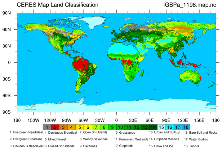
vegland_1.ncl: The following IGBP vegetation classification is derived from the CERES 10-min Map Land Classification.

Surface types 1 - 17 correspond to those defined by IGBP (International Geosphere Biosphere Programme). The last 3 surface types were defined for CERES. Surface type 18, Tundra, occurs when a location has an IGBP surface type of 16 (bare soil and rocks) and the Olson vegetation map identifies the same location as Tundra. Fresh snow, number 19, and sea ice, number 20 are not permanent surface types. They are obtained daily from the National Snow and Ice Data Center. The IGBP surface type for snow and ice number 15, is for permanent snow and ice. It does not change with time The IGBPa_1198.map does NOT show surface types 19 and 20 as these change daily. THIS MAP IS STATIC (i.e., doesn't change with time). For surface type maps that change with time, see MODIS Land products.

The third frame is identical to the first one, except the vegetation_modis color map, added in NCL V6.5.0, was used.

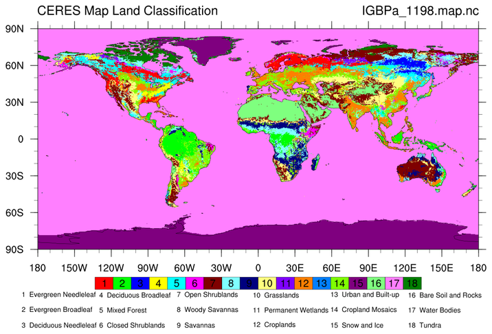
vegland_2.ncl: This is a high resolution (3600x7200) from a different source. A custom color map is created. Each color must match each category. This is slow when doing the full (global resolution).

vegland_3.ncl: This is the same as the previous example but only a region is selected and plotted. This is reasonably fast.

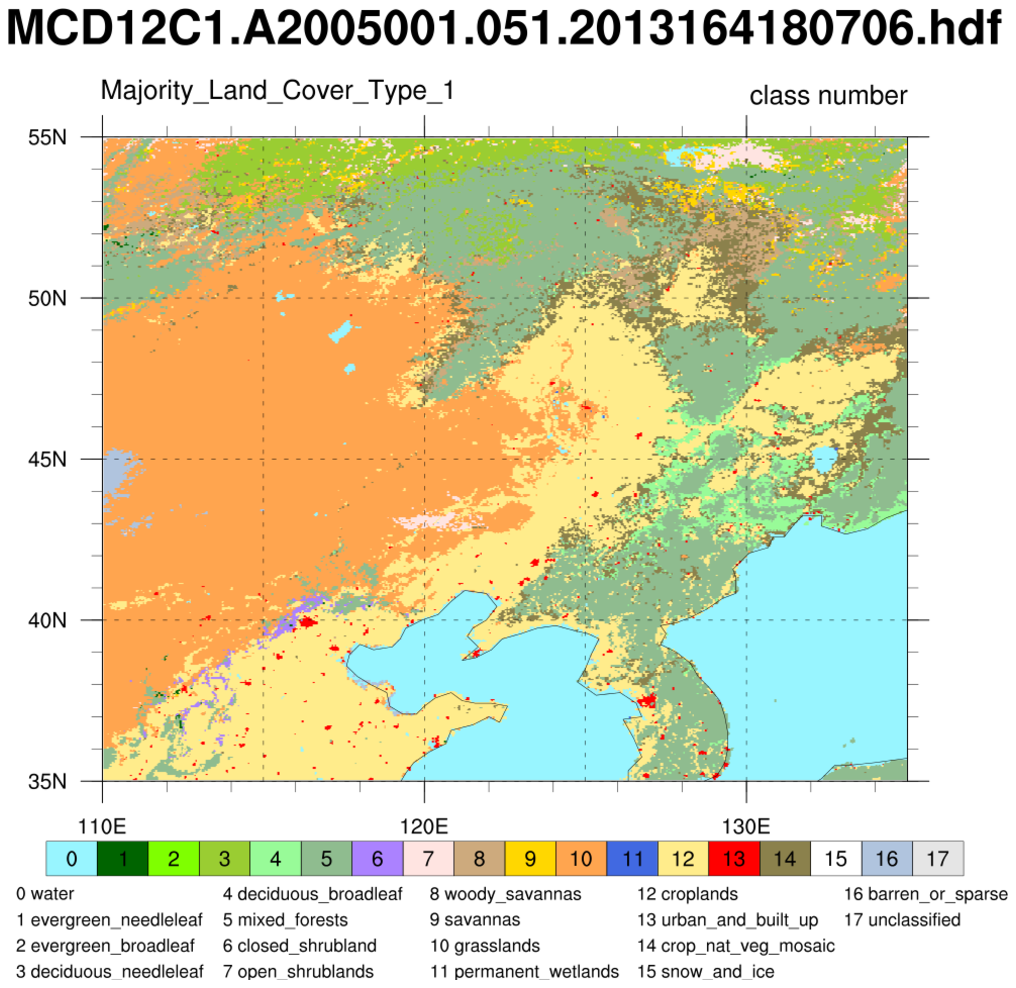
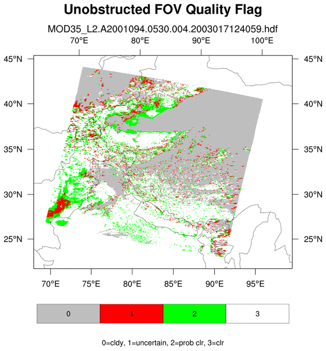hdf4eos_5.ncl: Illustrates the use of dim_gbits to extract bits. It also demonstrates explicitly labeling different colors with a specific integers.

The use of res@trGridType="TriangularMesh" makes the plotting faster.

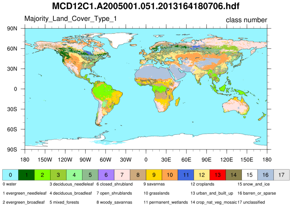
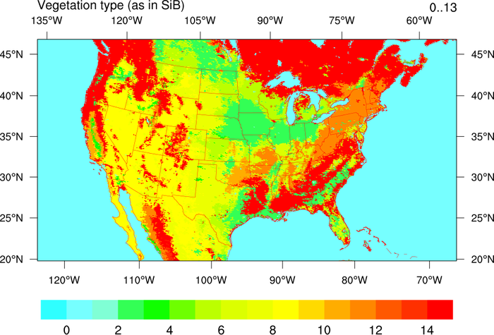raster_3.ncl: This vegetation raster plot is generated using 2-dimensional latitude and longitude coordinate values. These values are attached as attributes to the data (veg@lat2d and veg@lon2d), since traditional coordinate array syntax can't be used (these have to be 1-dimensional).

The gsnRightStringOrthogonalPosF and gsnLeftStringOrthogonalPosF resources are used to move the two subtitles up from the plot.

Generally, it is best to not use a 'smooth' color scheme for classification data because the categories are arbitrary.

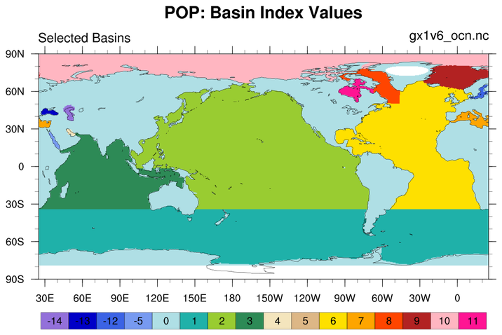popmask_1.ncl: Show selected POP Basins.

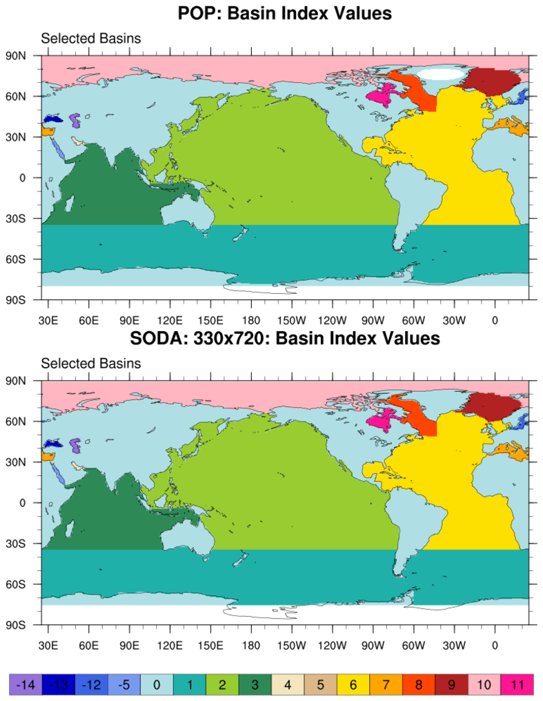popmask_3.ncl: Derive a mask for the SODA dataset using the POP REGION_MASK varaible. The REGION_MASK variable is categorical so a nearest neighbor approach is used. Several NCL functions are used to reduce the computational load. Only a subset set of distance calculations are performed. A netCDF file is created and a plot illustrating the original and derived region mask is generated. This took about 300 seconds on a MAC.

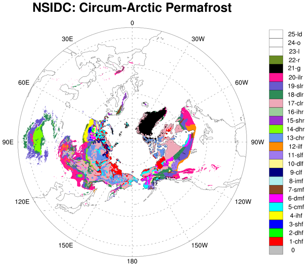permafrost_1.ncl: This figure is derived from a data file downloaded from NSIDC's Circum-Arctic Map of Permafrost and Ground Ice Conditions. It shows a circum-Arctic map of permafrost and ground ice conditions (12.5 km EASE grid). The source is the binary raster file "nhipa.byte". The numeric values and textual codes refer to different conditions. EG: "1-chf" indicates "Continuous permafrost extent with high ground ice content and thick overburden." Details are at the NSIDC site.

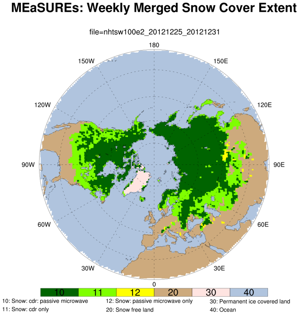ease_2.ncl: This plots discrete (categorical) snow extent data for Dec 25-31, 2012 rendered on a 100km resolution EASE grid.

The trick of using 'cnLevels' one greater than the actual values was neeeded to get the figure.