NCL Graphics: Geodesic Mesh

The geodesic meshes used in the examples on this page form a connection of lines over a sphere. The meshes are defined by a number of cells (ncells), each which of which have a certain number of edges defined by a set of vertices (nvert).

To contour data on a mesh, you must define the cell centers by either setting the sfXArray and sfYArray resources to one-dimensional arrays that represent the cell centers, or, if this is data to be plotted over a map, then by attaching the lat/lon centers of the data as special "lat1d" and "lon1d" attributes to the data being plotted.

When NCL encounters one-dimensional coordinates in this fashion, then under the hood it first converts the data to a triangular mesh before contouring it.

In addition, if your data has 2D arrays that define its cell edges (ncells x nvertices), then you can set the additional resources sfXCellBounds and sfYCellBounds to these arrays, which will likely produce a better looking contour plot.

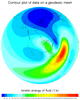
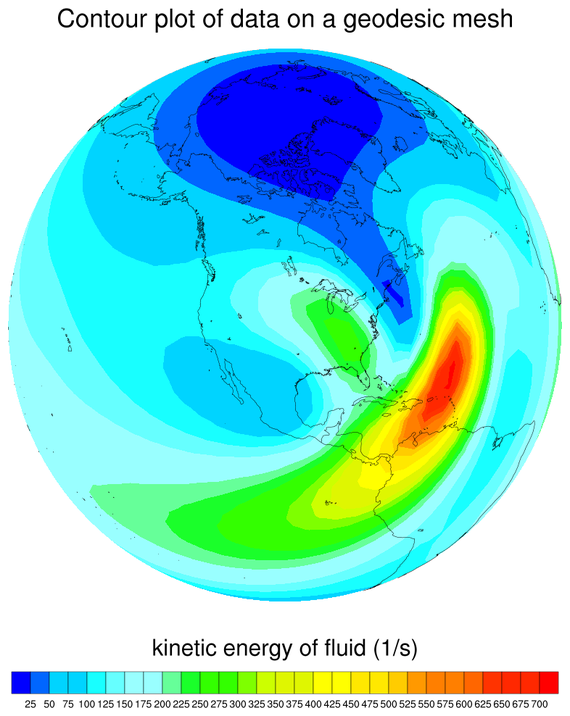
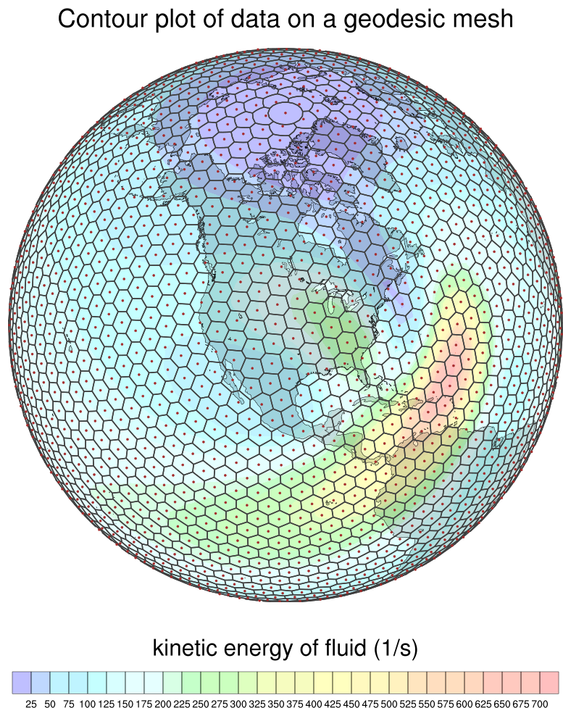
geo_1.ncl: This particular geodesic grid has 2562 cells, each with 5 edges. The lat/lon cell centers are defined as 1D arrays called grid_center_lat and grid_center_lon on the file, while the cell edges are defined as 2D arrays dimensioned 2562 x 6 (ncells x nvertices), called grid_corner_lat and grid_corner_lon.

To plot this data over a map, sfXArray and sfYArray are set to the mesh centers (grid_center_lat and grid_center_lon), while sfXCellBounds and sfYCellBounds are set to the cell corners (grid_corner_lat and grid_corner_lon). Both sets of lat/lon arrays are in radians, so they have to first be converted to degrees.

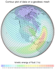
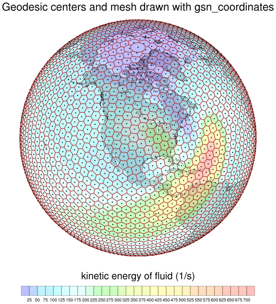
The second image draws the cell centers as filled dots, and the geodesic mesh as polylines. Note that the cell edges have to first be closed before drawing them.

See the next example which uses an updated version of gsn_coordinates to draw the mesh edges and centers.

geo_1_660.ncl: This image is similar to the second image from the previous example, except it uses a newer version of gsn_coordinates to draw the mesh edges and cell centers. You must have NCL version 6.6.0 or later for this functionality.

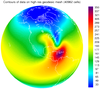
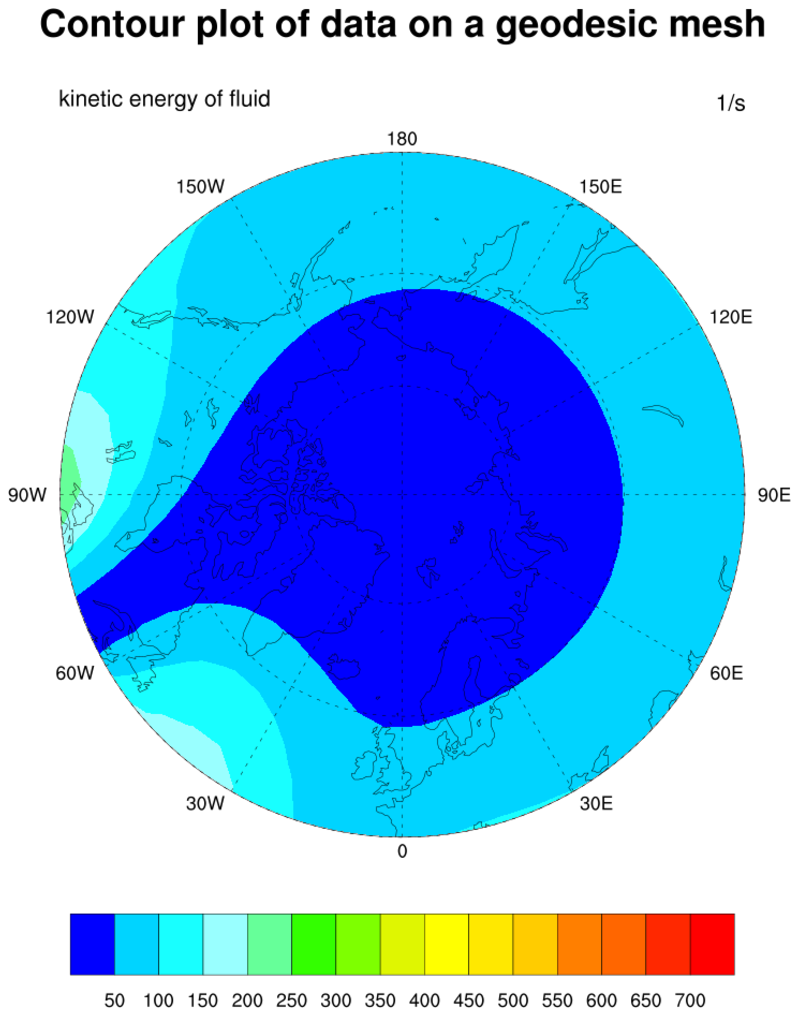
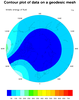geo_2.ncl: This script plots the same data as the previous examples, except over a polar stereographic plot of the northern hemisphere. Setting gsnPolar to either "NH" or "SH" selects the hemisphere, while mpMinLatF adjusts the minimum latitude (defaults to 0.0). If plotting over the southern hemisphere, then set mpMaxLatF to set the maximum latitude (defaults to 0.0).

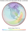
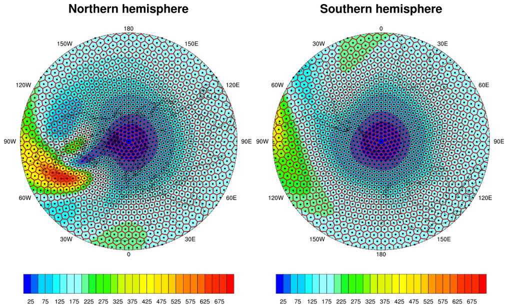
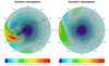geo_3.ncl: This script compares geodesic data drawn over both the northern and southern hemispheres using a panel plot created with gsn_panel.

gsn_coordinates is again used to draw he cell centers edges, except this time the special resource gsnCoordsAttach is set to True, telling the procedure to attach the lines and markers to the plots. This enables the plots to still contain the lines and markers when they are paneled later.

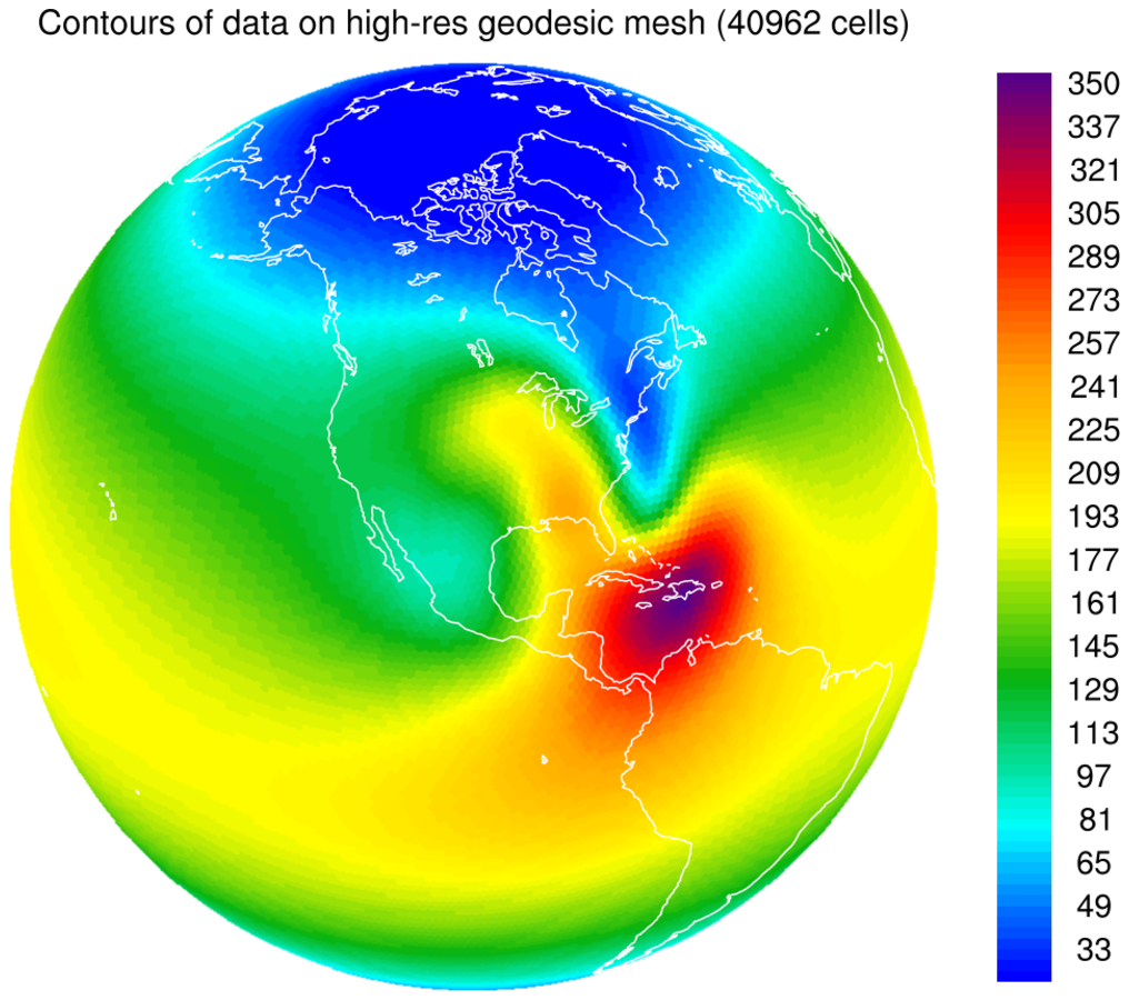
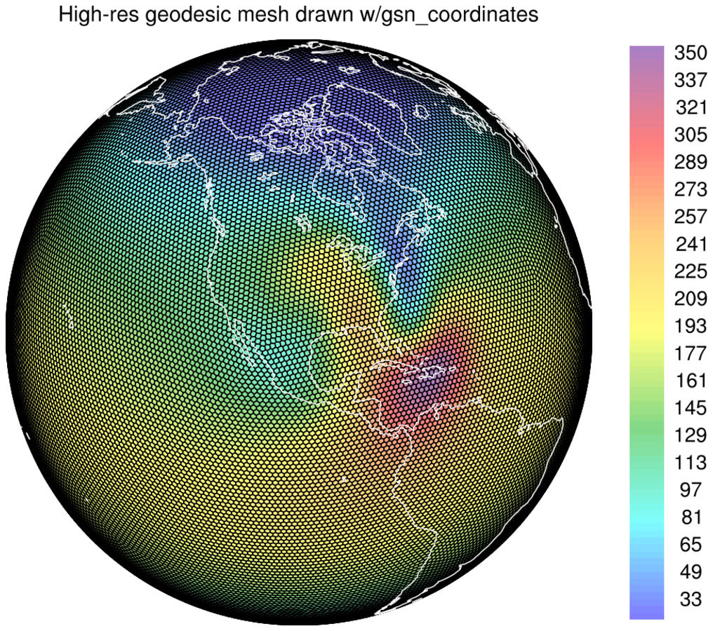
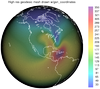geo_4.ncl: This script plot data over a higher resolution geodesic mesh (40962 cells) and adds just the cell edges using gsn_coordinates.

Note the cell centers are not drawn because the plot would be too busy otherwise. This is accomplished by using (/ and /) when passing "ke" to gsn_coordinates. This effectively strips the special lat1d and lon1d attributes from the variable, which prevents any cell center information from being passed to the procedure.